Quick Start - Object Detection with LTDETRv2 (NEW)
This guide demonstrates how to use LightlyTrain for object detection with our state-of-the-art LTDETRv2 model.
Installation
pip install lightly-train
Important
LightlyTrain is officially supported on:
Linux: CPU or CUDA
MacOS: CPU only
Windows (experimental): CPU or CUDA
We are planning to support MPS for MacOS.
Check the installation instructions for more details.
Predict using LightlyTrain’s LTDETR weights
Download an example image
Download an example image for inference:
wget -O image.jpg http://images.cocodataset.org/val2017/000000577932.jpg
Load the model weights
Load the model with LightlyTrain’s load_model function. This will automatically
download the model weights and load the model:
import lightly_train

model = lightly_train.load_model("ltdetrv2-s-coco")
Predict the objects
Run model.predict on the image. The method accepts file paths, URLs, PIL Images, or
tensors as input:
results = model.predict("image.jpg")
results["labels"]   # Class labels, tensor of shape (num_boxes,)
results["bboxes"]   # Bounding boxes in (xmin, ymin, xmax, ymax) absolute pixel
                    # coordinates of the original image. Tensor of shape (num_boxes, 4).
results["scores"]   # Confidence scores, tensor of shape (num_boxes,)
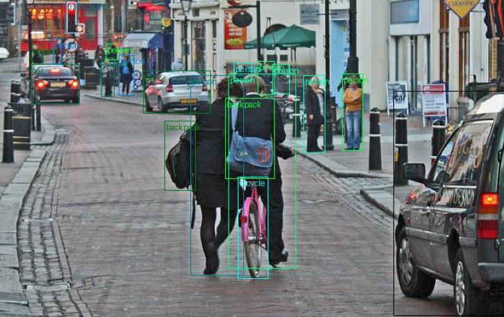
Visualize the results
Visualize the image and results to check what objects were detected:
import matplotlib.pyplot as plt
from torchvision.io import read_image
from torchvision.utils import draw_bounding_boxes

image = read_image("image.jpg")
image_with_boxes = draw_bounding_boxes(
    image,
    boxes=results["bboxes"],
    labels=[model.classes[label.item()] for label in results["labels"]],
)
plt.imshow(image_with_boxes.permute(1, 2, 0))
plt.show()
Train an LTDETR model
Training your own LTDETR model is straightforward with LightlyTrain.
Download a dataset
First download a dataset. The dataset must be in YOLO format, see the documentation for more details. You can use labelformat to convert any dataset to the YOLO format:
wget https://github.com/lightly-ai/coco128_yolo/releases/download/v0.0.1/coco128_yolo.zip && unzip -q coco128_yolo.zip
The dataset looks like this after the download completes:
coco128_yolo
├── images
│   ├── train2017
│   │   ├── 000000000009.jpg
│   │   ├── 000000000025.jpg
│   │   ├── ...
│   │   └── 000000000650.jpg
│   └── val2017
│       ├── 000000000139.jpg
│       ├── 000000000285.jpg
│       ├── ...
│       └── 000000013201.jpg
└── labels
    ├── train2017
    │   ├── 000000000009.txt
    │   ├── 000000000025.txt
    │   ├── ...
    │   └── 000000000659.txt
    └── val2017
        ├── 000000000139.txt
        ├── 000000000285.txt
        ├── ...
        └── 000000013201.txt
Start training
Next, start the training with the train_object_detection function. You only have to
specify the output directory, model, and input data. LightlyTrain automatically sets
the remaining training parameters and applies image augmentations. Of course you can
always customize these settings if needed:
import lightly_train

lightly_train.train_object_detection(
    out="out/my_experiment",
    model="ltdetrv2-s-coco",
    steps=100,  # Small number of steps for demonstration, default is 266_112.
    batch_size=4,  # Small batch size for demonstration, default is 32.
    data={
        "path": "coco128_yolo",
        "train": "images/train2017",
        "val": "images/val2017",
        "names": {
            0: "person",
            1: "bicycle",
            2: "car",
            3: "motorcycle",
            4: "airplane",
            5: "bus",
            6: "train",
            7: "truck",
            8: "boat",
            9: "traffic light",
            10: "fire hydrant",
            11: "stop sign",
            12: "parking meter",
            13: "bench",
            14: "bird",
            15: "cat",
            16: "dog",
            17: "horse",
            18: "sheep",
            19: "cow",
            20: "elephant",
            21: "bear",
            22: "zebra",
            23: "giraffe",
            24: "backpack",
            25: "umbrella",
            26: "handbag",
            27: "tie",
            28: "suitcase",
            29: "frisbee",
            30: "skis",
            31: "snowboard",
            32: "sports ball",
            33: "kite",
            34: "baseball bat",
            35: "baseball glove",
            36: "skateboard",
            37: "surfboard",
            38: "tennis racket",
            39: "bottle",
            40: "wine glass",
            41: "cup",
            42: "fork",
            43: "knife",
            44: "spoon",
            45: "bowl",
            46: "banana",
            47: "apple",
            48: "sandwich",
            49: "orange",
            50: "broccoli",
            51: "carrot",
            52: "hot dog",
            53: "pizza",
            54: "donut",
            55: "cake",
            56: "chair",
            57: "couch",
            58: "potted plant",
            59: "bed",
            60: "dining table",
            61: "toilet",
            62: "tv",
            63: "laptop",
            64: "mouse",
            65: "remote",
            66: "keyboard",
            67: "cell phone",
            68: "microwave",
            69: "oven",
            70: "toaster",
            71: "sink",
            72: "refrigerator",
            73: "book",
            74: "clock",
            75: "vase",
            76: "scissors",
            77: "teddy bear",
            78: "hair drier",
            79: "toothbrush",
        },
    },
)
Once the training is complete, the output directory looks like this:
out/my_experiment
├── checkpoints
│   ├── best.ckpt
│   └── last.ckpt
├── events.out.tfevents.1764251158.ef9b159fe4b8.273.0
├── exported_models
│   ├── exported_best.pt
│   └── exported_last.pt
└── train.log
The best model checkpoint is saved to
out/my_experiment/exported_models/exported_best.pt.
Predict with your own LTDETR weights
Load the model weights
model = lightly_train.load_model("out/my_experiment/exported_models/exported_best.pt")
Predict the objects
results = model.predict("image.jpg")

results["labels"]   # Class labels, tensor of shape (num_boxes,)
results["bboxes"]   # Bounding boxes in (xmin, ymin, xmax, ymax) absolute pixel
                    # coordinates of the original image. Tensor of shape (num_boxes, 4).
results["scores"]   # Confidence scores, tensor of shape (num_boxes,)
Visualize the results
image = read_image("image.jpg")
image_with_boxes = draw_bounding_boxes(
    image,
    boxes=results["bboxes"],
    labels=[model.classes[label.item()] for label in results["labels"]],
)
plt.imshow(image_with_boxes.permute(1, 2, 0))
plt.show()
Benchmark your checkpoint
You can use the benchmark_object_detection (in beta) command to measure the inference
performance of an object detection model on a validation dataset.
result = lightly_train.benchmark_object_detection(
    out="out/my_benchmark",
    dataset_name="coco128",  # Human-readable name shown in the report.
    model="out/my_experiment/exported_models/exported_best.pt",
    data={
        "path": "coco128_yolo",
        "train": "images/train2017",
        "val": "images/val2017",
        "names": {
            0: "person",
            1: "bicycle",
            2: "car",
            3: "motorcycle",
            4: "airplane",
            5: "bus",
            6: "train",
            7: "truck",
            8: "boat",
            9: "traffic light",
            10: "fire hydrant",
            11: "stop sign",
            12: "parking meter",
            13: "bench",
            14: "bird",
            15: "cat",
            16: "dog",
            17: "horse",
            18: "sheep",
            19: "cow",
            20: "elephant",
            21: "bear",
            22: "zebra",
            23: "giraffe",
            24: "backpack",
            25: "umbrella",
            26: "handbag",
            27: "tie",
            28: "suitcase",
            29: "frisbee",
            30: "skis",
            31: "snowboard",
            32: "sports ball",
            33: "kite",
            34: "baseball bat",
            35: "baseball glove",
            36: "skateboard",
            37: "surfboard",
            38: "tennis racket",
            39: "bottle",
            40: "wine glass",
            41: "cup",
            42: "fork",
            43: "knife",
            44: "spoon",
            45: "bowl",
            46: "banana",
            47: "apple",
            48: "sandwich",
            49: "orange",
            50: "broccoli",
            51: "carrot",
            52: "hot dog",
            53: "pizza",
            54: "donut",
            55: "cake",
            56: "chair",
            57: "couch",
            58: "potted plant",
            59: "bed",
            60: "dining table",
            61: "toilet",
            62: "tv",
            63: "laptop",
            64: "mouse",
            65: "remote",
            66: "keyboard",
            67: "cell phone",
            68: "microwave",
            69: "oven",
            70: "toaster",
            71: "sink",
            72: "refrigerator",
            73: "book",
            74: "clock",
            75: "vase",
            76: "scissors",
            77: "teddy bear",
            78: "hair drier",
            79: "toothbrush",
        },
    },
)

result.print()
The command returns a BenchmarkResult instance and writes two files to the out
directory:
out/my_benchmark
├── benchmark_results.json
└── benchmark_summary.md
benchmark_results.json: the full result as JSON.benchmark_summary.md: a human-readable Markdown report.
The report (also available via result.to_markdown()) contains the run configuration,
device info, performance metrics, and a throughput & latency table.
Next Steps
Object Detection Documentation: If you want to learn more about object detection with LightlyTrain.