Embedding Model for Satellite Images with Torchvision’s ResNet
![]()
This tutorial demonstrates how to train an embedding model with LightlyTrain on unlabeled data. The model is then used to generate embeddings from the images and visualize them in 2D. Embedding models are useful for a variety of tasks such as:
Image retrieval
Clustering
Outlier detection
Dataset curation
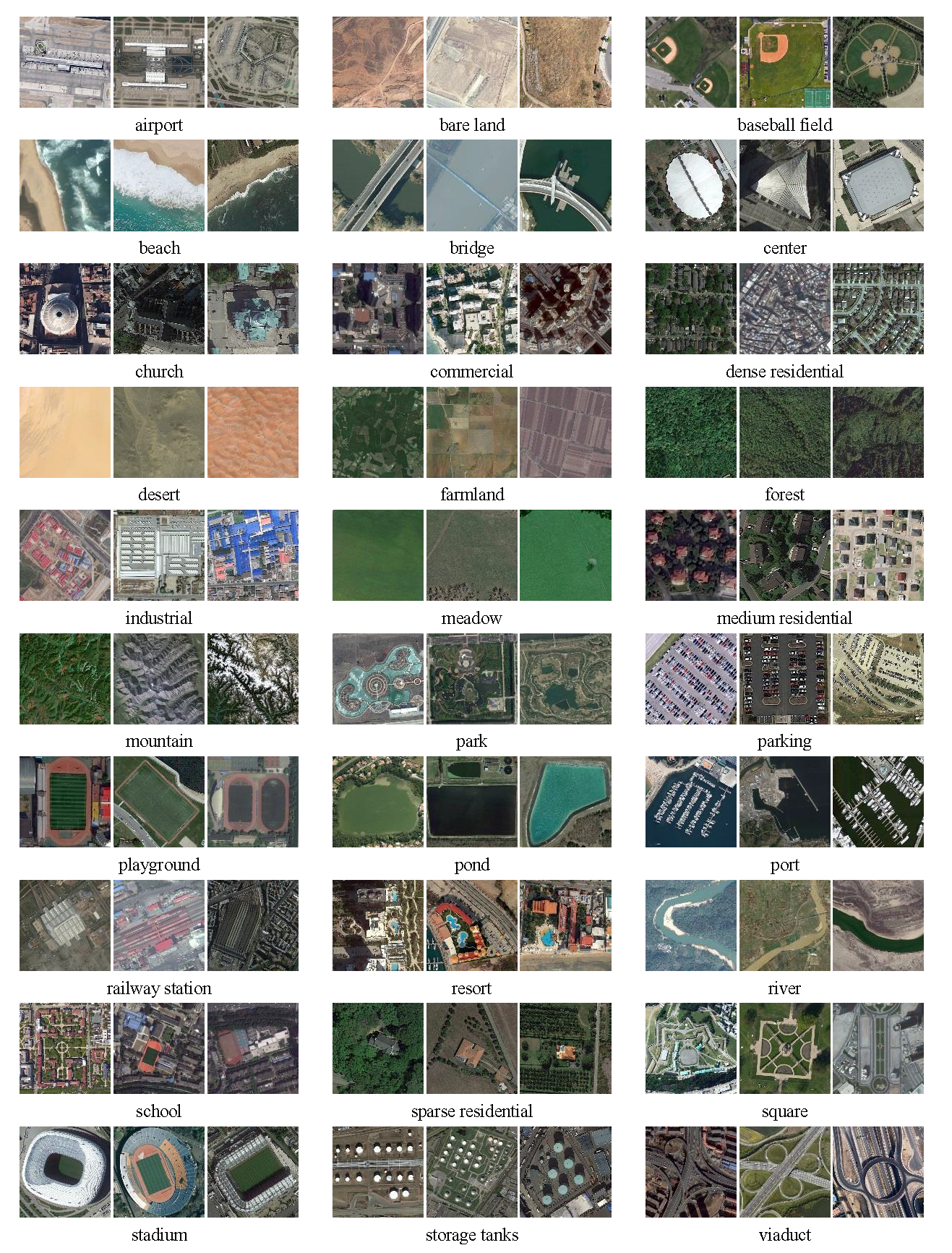
For this tutorial we will use the Aerial Image Dataset (AID) which contains 30,000 satellite images from Google Earth grouped into 30 classes.
Install the Dependencies
To get started, we first need to install the required dependencies:
lightly-trainto train the embedding model and generate the embeddingsumap-learnto reduce the dimensionality of the embeddings for visualization
pip install lightly-train umap-learn
Download the Dataset
Next, we have to download the AID dataset:
wget https://www.kaggle.com/api/v1/datasets/download/jiayuanchengala/aid-scene-classification-datasets
unzip aid-scene-classification-datasets
After unzipping, the dataset looks like this:
AID
├── Airport
│   ├── airport_100.jpg
│   ├── ...
│   └── airport_9.jpg
├── BareLand
│   ├── bareland_100.jpg
│   ├── ...
│   └── bareland_9.jpg
├── ...
└── Viaduct
    ├── viaduct_100.jpg
    ├── ...
    └── viaduct_9.jpg
The images are grouped by class into subdirectories. LightlyTrain doesn’t need the class information for training, but we will use it later to check the quality of the learned embeddings.
Train the Embedding Model
Once the data is downloaded, we can start training the embedding model. We will use
a lightweight ResNet18 model from torchvision for this. We also use bf16-mixed precision
to speed up training. If your GPU does not support mixed precision, you can remove the
precision argument.
Training for 1000 epochs on a single RTX 4090 GPU takes about 5 hours. If you don’t want to wait that long, you can reduce the number of epochs to 100. This will result in lower embedding quality, but only takes 30 minutes to complete.
import lightly_train

if __name__ == "__main__":
    lightly_train.train(
        out="out/aid_resnet18_lightly_train",
        data="AID",
        model="torchvision/resnet18",
        epochs=1000,
        precision="bf16-mixed",
    )
Embed the Images
Once the model is trained, we can use it to generate embeddings for the images. We will
save the embeddings to a file called embeddings_lightly_train.pt.
import lightly_train

if __name__ == "__main__":
    lightly_train.embed(
        out="embeddings_lightly_train.pt",
        data="AID",
        checkpoint="out/aid_resnet18_lightly_train/checkpoints/last.ckpt",
    )
Visualize the Embeddings
Now that we have the embeddings, we can visualize them in 2D with UMAP. UMAP is a dimension reduction technique that is well suited for visualizing high-dimensional data.
import matplotlib.pyplot as plt
import torch
import umap

# Load the embeddings
data = torch.load("embeddings_lightly_train.pt", weights_only=True, map_location="cpu")
embeddings = data["embeddings"]
filenames = data["filenames"]

# Reduce dimensions with UMAP
reducer = umap.UMAP()
embedding_2d = reducer.fit_transform(embeddings)

# Plot
plt.figure(figsize=(10, 8))
plt.scatter(embedding_2d[:, 0], embedding_2d[:, 1], s=5)
plt.title("UMAP of LightlyTrain Embeddings")
plt.show()
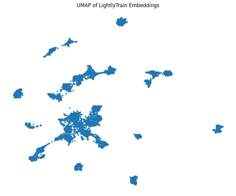
Visualization of the learned embeddings projected into 2D space with UMAP.
We can see that the embeddings are nicely separated into well-defined clusters. Such visualizations are extremely useful when curating a dataset. They can quickly give you an overview of your data including outliers and duplicates. Furthermore, the clusters can be used to efficiently label your dataset.
Color the Clusters
Let’s check if the clusters make sense by coloring them according to the class labels
that are available in this dataset. All filenames have the format <class>/<image_name>.jpg
which lets us extract the class labels easily. Let’s plot the embeddings again:
import matplotlib.pyplot as plt

# Color embeddings based on class labels
class_name_to_id = {class_name: i for i, class_name in enumerate({filename.split("/")[0] for filename in filenames})}
filename_to_class_id = {filename: class_name_to_id[filename.split("/")[0]] for filename in filenames}
color = [filename_to_class_id[filename] for filename in filenames]

# Plot
plt.figure(figsize=(10, 8))
plt.scatter(embedding_2d[:, 0], embedding_2d[:, 1], s=5, c=color, cmap="tab20")
plt.title("UMAP of LightlyTrain Embeddings Colored by Class")
plt.show()
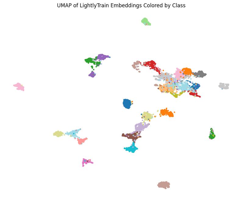
Embeddings colored by ground truth class labels.
The embeddings are well separated by class with few outliers. The LightlyTrain model has learned meaningful embeddings without using any class information! For reference, we show a comparison to embeddings generated with an ImageNet supervised pretrained model below:
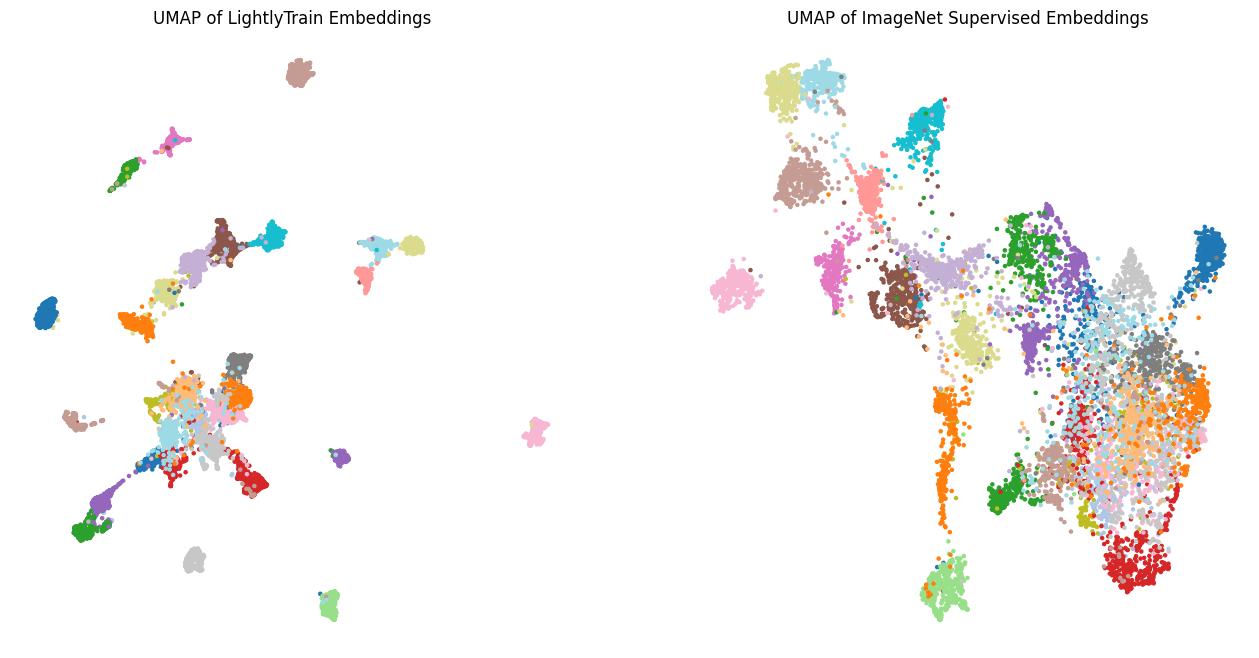
Comparison between embeddings generated with LightlyTrain and a supervised ImageNet pretrained model.
We can see that the clusters from the LightlyTrain embeddings are much more compact and have fewer overlaps. This means that the model has learned better representations and will make fewer mistakes for embedding-based tasks like image retrieval or clustering. This highlights how training an embedding model on the target dataset can improve the embeddings quality compared to using an off-the-shelf embedding model.
Conclusion
In this tutorial we have learned how to train an embedding model using unlabeled data with LightlyTrain. We have also seen how to visualize the embeddings with UMAP and color them according to class labels. The visualizations show that the model has learned strong embeddings that capture the information of the images well and group similar images together. This is a great starting point for fine-tuning or any embedding-based task such as image retrieval, clustering, outlier detection or dataset curation.