Explore LightlyTrain embeddings in LightlyStudio
In this tutorial, you distill a large embedding model into a small one with LightlyTrain. Then you explore and curate the result in LightlyStudio.
You will:
- Distill a large pretrained model into a small one, with LightlyTrain and no labels.
- Export the small model and run it inside LightlyStudio to embed your data.
- Explore the 2D embedding plot to find clusters, outliers, and near-duplicates.
- Select a diverse subset for labeling or training.
Why distill a model on your own images
A small model is cheap to run. On fine-grained data it is also weak, because it does not have the capacity to separate classes that look alike.
A large model separates those classes. It also costs much more to run for every image you embed.
Distillation gives you both. LightlyTrain copies the behavior of the large model into the small one, on your own unlabeled images. You keep the inference cost of the small model.
This tutorial uses CUB-200-2011, a dataset of 11,788 photos of 200 bird species. Species recognition is fine-grained, so model capacity matters here.
The table gives the k-nearest-neighbor class purity for each model. Purity is the fraction of the 10 nearest neighbors of an image that have the same species. The first row is the floor: pick neighbors at random and 1 in 200 lands on the same species.
| Model | Parameters | Purity |
|---|---|---|
| Random neighbors (the floor, no model) | — | 0.005 |
| DINOv3 ViT-T, off the shelf (distilled by Lightly) | 5.5M | 0.081 |
| MobileCLIP (LightlyStudio default) | 11M | 0.357 |
| DINOv3 ViT-S | 21.6M | 0.582 |
| DINOv3 ViT-T, distilled in this tutorial | 5.5M | 0.606 |
| DINOv3 ViT-B (the teacher) | 85.7M | 0.715 |
| DINOv3 ViT-L | 303.2M | 0.777 |
The distilled ViT-T closes 83% of the distance to its teacher. The teacher is 15 times larger. The distilled ViT-T also scores higher than an off-the-shelf ViT-S, which is 4 times larger.
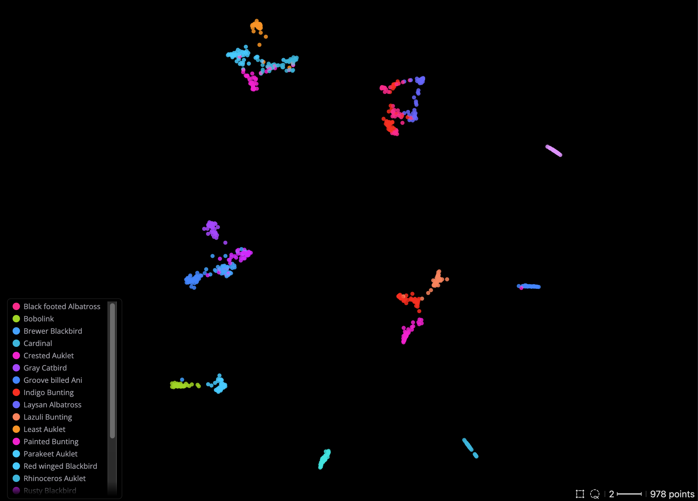
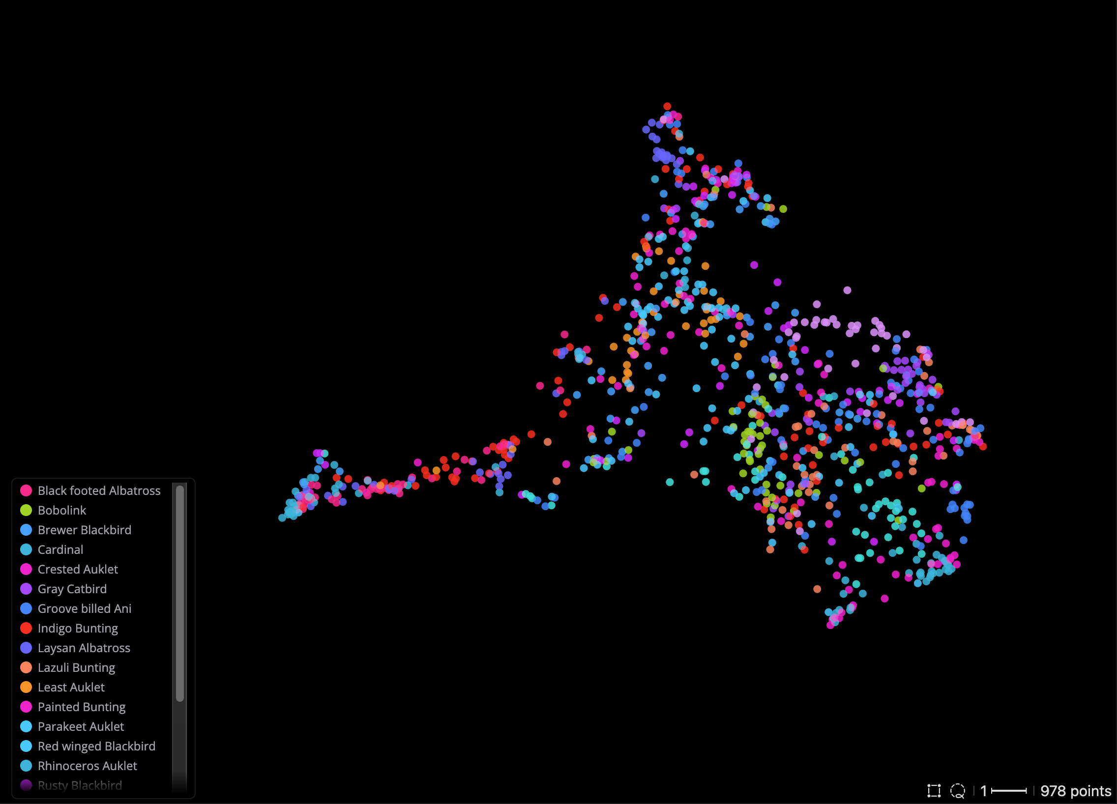
The next two plots show the same 978 images from 20 species, colored by species. The model is the same size in both. Only the weights are different. Step 4 loads this same slice, so the right-hand plot is the one you get at the end of this tutorial. The distillation itself still runs on all 200 species.
The purity in each caption is measured on these 978 images from 20 species. The table above measures all 200 species instead. Fewer species is an easier task, so the caption values are higher. Both use the same metric.
Pick a dataset where a larger model helps
Distillation moves the knowledge of the teacher into the student. If a large model scores about the same as a small one on your data, there is nothing to move. On CUB-200, ViT-L scores 0.195 above ViT-S, so there is a large margin to recover. On coarse-grained data, where a small model already comes close to a large one, distillation gives almost nothing.
How the workflow fits together
LightlyTrain and LightlyStudio meet at one point: the embedding model.
- Distill a large model into a small one with LightlyTrain.
- Export the small model as a torch module.
- Load the module into LightlyStudio, which runs it to embed your data.
- Explore and curate the embeddings in the 2D plot.
This tutorial builds two small scripts. train_and_export.py runs the distillation once. explore.py loads the model into LightlyStudio, and you can run it any time. Runnable versions of both are on GitHub: example_lightlytrain_train_and_export.py and example_lightlytrain_explore.py.
Prerequisites
To follow this tutorial, make sure that you have:
- Python 3.10 or newer. Step 1 passes
filtertotarfile.extractall, which on 3.10 and 3.11 needs a patch release from June 2023 or later. - A GPU for the distillation step. On 2 NVIDIA RTX 4090 GPUs, the run in this tutorial takes about 21 minutes.
- A CUDA GPU, Apple Silicon (MPS), or a CPU for the exploration step
- About 4 GB of free disk space
Installation
LightlyTrain and LightlyStudio are separate packages. Install both:
pip install lightly-train lightly-studio
Step 1: Get a dataset
Create the first script, train_and_export.py. This script downloads CUB-200-2011. The dataset has one folder for each species, and the explore script reads those folder names to label each image.
To use your own data, point IMAGE_PATH at a folder that holds one subfolder for each class, with the images directly inside. That is the layout explore.py reads in Step 4, and the only one it accepts. IMAGE_PATH is defined in both scripts, so change it in both. See Load an Image Dataset.
Each step below writes one function. Step 5 calls them.
import tarfile
from pathlib import Path

import lightly_train

from lightly_studio.dataset import file_utils

CUB_URL = "https://data.caltech.edu/records/65de6-vp158/files/CUB_200_2011.tgz"
ARCHIVE = Path("CUB_200_2011.tgz")
# The archive also holds a top-level attributes.txt, so extract into a directory of
# our own instead of the working directory.
DATA_DIR = Path("data")
# Touched only after extractall returns. CUB_200_2011/images appears three members
# into the archive, so its presence says nothing about whether extraction finished.
EXTRACT_DONE = DATA_DIR / ".extracted"
IMAGE_PATH = DATA_DIR / "CUB_200_2011" / "images"


def download_dataset() -> None:
    # The helper downloads to a temp file and moves it into place only on success,
    # so an interrupted download is never mistaken for a complete one.
    file_utils.download_file_if_does_not_exist(url=CUB_URL, local_filename=ARCHIVE)
    if not EXTRACT_DONE.exists():
        with tarfile.open(ARCHIVE) as tar:
            # filter="data" refuses members that would write outside DATA_DIR.
            tar.extractall(DATA_DIR, filter="data")
        EXTRACT_DONE.touch()
Step 2: Distill the model
Distillation copies the behavior of a large teacher into a small student. It uses no labels.
Here the student is dinov3/vitt16 and the teacher is dinov3/vitb16. Both start from pretrained weights. Both are covered by the DINOv3 license, which the model you export inherits. For Apache 2.0 weights, use a DINOv2 model instead.
def distill() -> None:
    lightly_train.pretrain(
        out="out/pretrain",
        data=IMAGE_PATH,
        model="dinov3/vitt16",  # The student. This is the model you run later.
        method="distillation",
        method_args={"teacher": "dinov3/vitb16"},  # The teacher. Larger and stronger.
        epochs=100,
        # Pick a crashed run back up instead of repeating all 100 epochs. On a first
        # run there is no checkpoint and this does nothing.
        resume_interrupted=True,
    )
Training writes a checkpoint to out/pretrain/checkpoints/last.ckpt.
The student is already a distilled model
Lightly trained the dinov3/vitt16 weights, not Meta. They come from an earlier distillation run, with DINOv3 ViT-L/16 as the teacher and ImageNet-1K as the data. This tutorial distills that model again, onto one specific dataset. So the 0.081 score in the table above is a general-purpose model on fine-grained birds, not an untrained one. The floor is 0.005.
Any name from lightly_train.list_models() works for model and for teacher. See the supported models of LightlyTrain. For other methods, see the pretraining guide and the available methods.
Step 3: Export the embedding model
Export the student as a plain torch module. LightlyStudio loads this file and runs it directly.
def export_student() -> None:
    lightly_train.export(
        out="out/embedding_model.pt",
        checkpoint="out/pretrain/checkpoints/last.ckpt",
        part="embedding_model",
        format="torch_model",
        overwrite=True,
    )
Finish the script by calling the three functions. The __main__ guard is required: LightlyTrain starts dataloader workers that re-import this file on macOS and Windows, and without it the run crashes during startup.
if __name__ == "__main__":
    download_dataset()
    distill()
    export_student()
Step 4: Load the model into LightlyStudio
Now create the second script, explore.py. This script points at the images and loads the model that you exported. It registers an embedder that runs the model. LightlyStudio then embeds each sample during ingestion.
Beta API
The embeddings API is in beta. Its interface can change in future releases without a deprecation period.
Register the embedder before you create the dataset, so ingestion embeds with it.
from pathlib import Path

import torch
from PIL import Image
from torchvision import transforms

import lightly_studio as ls
from lightly_studio.core.annotation import CreateClassification
from lightly_studio.dataset import file_utils
from lightly_studio.embed import image_crop_embedding, image_embedding
from lightly_studio.embed.image_embedding import EmbeddingContext
from lightly_studio import EmbeddingResult
from lightly_studio_serve.embedder import (
    ImageCropPathEmbedder,
    ImagePathEmbedder,
    ImagePILEmbedder,
)

# train_and_export.py already downloaded CUB-200-2011 to data/CUB_200_2011/.
IMAGE_PATH = Path("data/CUB_200_2011/images")
# The plot gets one color per species, and 200 colors are hard to tell apart. These
# two settings load a smaller slice so the plot stays readable. Set both to None to
# load all 200 species and all 11,788 images.
NUM_SPECIES: int | None = 20
IMAGES_PER_SPECIES: int | None = 50

IMAGE_SIZE = 224
# LightlyTrain normalizes with ImageNet statistics by default.
IMAGENET_MEAN = (0.485, 0.456, 0.406)
IMAGENET_STD = (0.229, 0.224, 0.225)


class LightlyTrainEmbedder(ImagePathEmbedder, ImageCropPathEmbedder, ImagePILEmbedder):
    """Run a model exported from LightlyTrain to embed images on the fly.

    The model is vision-only, so this embedder does not subclass ``TextEmbedder``
    and text search stays off.
    """

    def __init__(self, model_file: str) -> None:
        # Auto select device: CUDA > MPS (Apple Silicon) > CPU.
        self._device = torch.device(
            "cuda"
            if torch.cuda.is_available()
            else "mps"
            if torch.backends.mps.is_available()
            else "cpu"
        )
        # map_location="cpu" first, so a model exported on a GPU still loads on a CPU/MPS host.
        self._model = torch.load(
            model_file, map_location="cpu", weights_only=False
        ).to(self._device).eval()
        self._preprocess = transforms.Compose(
            [
                transforms.Resize((IMAGE_SIZE, IMAGE_SIZE)),
                transforms.ToTensor(),
                transforms.Normalize(mean=IMAGENET_MEAN, std=IMAGENET_STD),
            ]
        )
        self._model_hash = file_utils.get_file_xxhash(Path(model_file))
        # EmbeddingModel.forward returns (B, D, 1, 1); infer D from a dummy pass.
        with torch.no_grad():
            dummy = torch.zeros(1, 3, IMAGE_SIZE, IMAGE_SIZE, device=self._device)
            self._dimension = int(self._model(dummy).flatten(1).shape[1])

    def embedding_space_spec(self) -> ls.EmbeddingSpaceSpec:
        return ls.EmbeddingSpaceSpec(
            space_key=f"lightlytrain/{self._model_hash}", dimension=self._dimension
        )

    def embed_images(self, paths: list[str]) -> EmbeddingResult:
        return image_embedding.embed_image_files_batched(
            filepaths=paths, context=self._context(), show_progress=True
        )

    def embed_image_crops(self, crops: list[ls.ImageCrop]) -> EmbeddingResult:
        return image_crop_embedding.embed_image_crops_batched(
            image_crops=crops, context=self._context(), show_progress=True
        )

    def embed_images_pil(self, images: list[Image.Image]) -> EmbeddingResult:
        return image_embedding.embed_pil_images_batched(
            images=images, context=self._context(), show_progress=False
        )

    def _context(self) -> EmbeddingContext:
        return EmbeddingContext(
            embedding_dimension=self._dimension,
            max_batch_size=128,
            device=self._device,
            preprocess=self._preprocess,
            encode_batch=lambda batch: self._model(batch).flatten(1).cpu().numpy(),
        )


# Check the inputs before connecting, because cleanup_existing=True below deletes the
# local database. Both paths are relative, so the usual mistake is the working directory.
for required_path in (IMAGE_PATH, Path("out/embedding_model.pt")):
    if not required_path.exists():
        raise SystemExit(
            f"{required_path} not found (cwd={Path.cwd()}). "
            "Run train_and_export.py first."
        )

# Resets the local database so a re-run starts clean. Remove to keep prior tags and curation.
ls.db_manager.connect(cleanup_existing=True)
ls.register_default_embedder(embedder=LightlyTrainEmbedder("out/embedding_model.pt"))

dataset = ls.ImageDataset.create(name="lightlytrain-embeddings")

# This script expects one subfolder per class with the images directly inside, the
# layout CUB-200-2011 ships. Anything else is rejected rather than loaded wrong.
species_dirs = sorted(p for p in IMAGE_PATH.iterdir() if p.is_dir() and p.name[0] != ".")
if not species_dirs:
    raise SystemExit(
        f"{IMAGE_PATH} has no class subfolders. For a flat folder of images, replace "
        "this block with a single dataset.add_images_from_path(path=IMAGE_PATH) call "
        "and drop the labelling loop below."
    )

# One call per species, so each species contributes at most IMAGES_PER_SPECIES images.
# A single call would cap the total across all species instead.
for species_dir in species_dirs[:NUM_SPECIES]:
    dataset.add_images_from_path(path=species_dir, limit=IMAGES_PER_SPECIES)

# Label each image with its species, so you can color the plot by species in the GUI.
# CUB folders look like "001.Black_footed_Albatross".
for sample in dataset:
    folder = Path(sample.file_path_abs).parent.name
    species = folder.split(".", 1)[-1].replace("_", " ")
    sample.add_annotation(
        CreateClassification(class_name=species), annotation_source="species"
    )
Match your training normalization
The transform above matches the ImageNet default of LightlyTrain. If you trained with custom normalize_args, pass the same mean and standard deviation.
Keep the same LightlyTrain version
torch.load(..., weights_only=False) unpickles the model class of LightlyTrain. The environment that runs LightlyStudio needs the same lightly-train version that you exported with. This load also runs code from the file. Load only model files that you trust.
Text search stays off, because the model has no text encoder. See Using your own embeddings and the Embeddings API for the full set of embedder capability interfaces.
Alternative: precompute the embeddings
To embed once, offline, run lightly_train.embed(...) to write vectors to a file. Then load them with the pattern in example_load_existing_embeddings.py. That path embeds whole images only.
Step 5: Explore the embedding map
Add one line to the end of explore.py to open the app:
ls.start_gui(open_browser=True)
Now run both scripts. Distill once, then explore:
python train_and_export.py   # distill and export the model (slow; run once)
python explore.py            # embed your data and open LightlyStudio
Click the Embed button in the top right to open the embedding plot. The plot shows every image as a point in a 2D projection (PaCMAP) of the embedding space. To color the points by species, open Color by at the bottom of the plot and pick annotations. You get the plot at the top of this page.
Read the map:
- Hover a point to preview its image.
- Look for clusters. Tight groups are visually similar images.
- Watch the edges. Points far from any cluster are outliers or wrong annotations.
- Spot near-duplicates. Points on top of each other are almost identical images.
Read the numbers, not only the plot
A 2D projection keeps local neighborhoods, not distances. Two different embedding spaces can give similar plots, so a plot on its own does not tell you which model is better. Every purity number on this page uses the 10 nearest neighbors by cosine similarity. The table uses 20 images from each of the 200 species. The two plot captions use the 978 images from 20 species, so their numbers are higher.
What the clusters contain
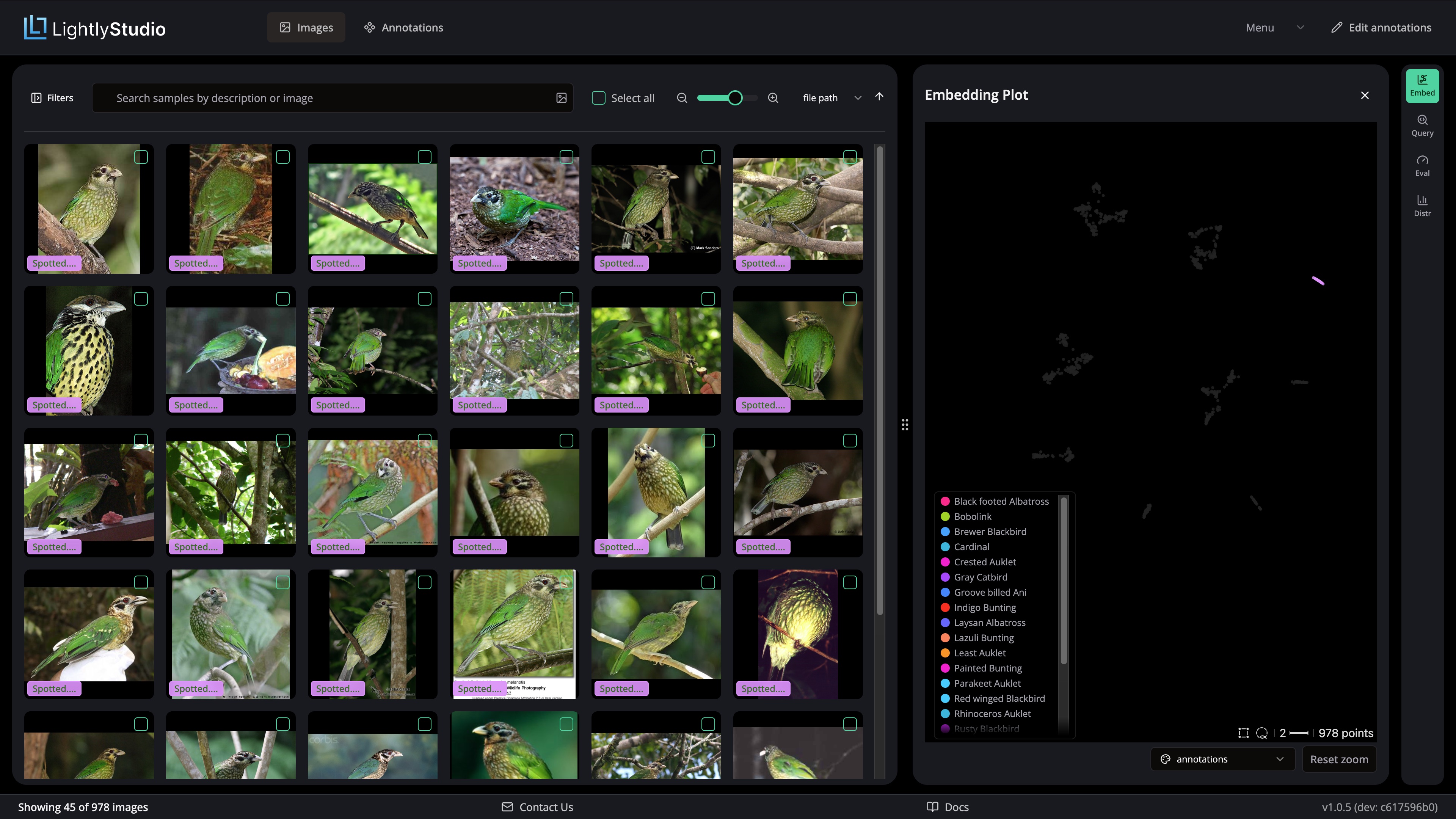
Lasso a tight cluster to scope the grid to its images, and it turns out to be one coherent group. The tightest clusters are close to a single species, with a few strays. Here are four of them:


Step 6: Select and curate a subset
The map is not only for looking. Turn what you see into a curated subset. A diversity selection picks samples from across the whole embedding space. A smaller labeling set then still covers the variety in your data.
Add this code to explore.py, before the ls.start_gui(...) line:
dataset.query().sampling().diverse(
    n_samples_to_select=32, sampling_result_tag_name="diverse_subset"
)
The result is saved as a tag. Open the tag in the grid to review the picks. You can also color the embedding plot by the tag to see the spread.
You can do the same by hand. Lasso a region in the plot to scope the grid to those samples, review them, and tag what you want to keep. Selection works in both directions. For every strategy, see Sampling.
Conclusion
In this tutorial, you distilled a large model into a small one with LightlyTrain, on unlabeled images. Then you ran the small model inside LightlyStudio to explore and curate your data.
The connection between the two products is a single model file. The distilled ViT-T went from 0.081 to 0.606 purity, at the inference cost of a 5.5M-parameter model.
After LightlyStudio loads the model file, the embedding plot and every sampling strategy work as they do with a built-in model. Text search is the one exception, because this model is vision-only.
To go further, distill on your full dataset, try a different teacher from lightly_train.list_models(), or read Embeddings and Sampling.
