Explore and annotate images with embeddings

In this tutorial, you explore the Imagenette dataset in LightlyStudio and use image similarity to guide labeling. Reviewing images one at a time is slow. Embeddings put similar images next to each other, so you can review a whole group at once and give all of its images the same annotation class in one action.

You will:

• Import 9,469 raw images across 10 classes.
• Explore the embedding plot, and use the lasso to select groups of similar images.
• Review a selected group and annotate all of it in one action.
• Use the legend and the Color by control to inspect your annotations.
• Load the ground truth of the dataset and measure your agreement with it.
• Export your work.

The finished dataset, with the embedding plot colored by annotation class.

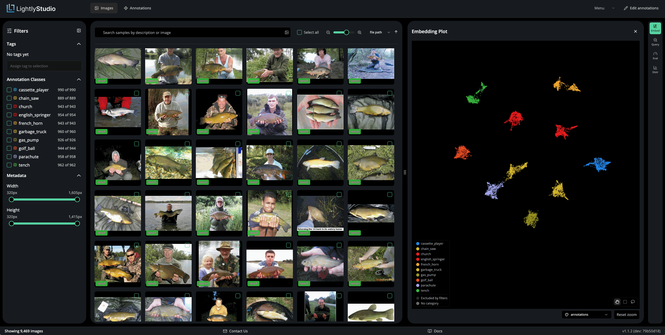
An embedding represents an image as a numerical vector. Images with similar visual or semantic content get nearby embeddings. LightlyStudio projects these vectors into a two-dimensional plot, where you can explore groups and inspect their images.

You do not need to annotate the entire dataset to finish this tutorial. Complete several groups, export your progress, and return to the remaining images later.

Step 1: Download the dataset

Imagenette is a subset of ImageNet with 10 classes, assembled by fast.ai. The classes are easy to tell apart, which makes the dataset a good fit for this workflow: you can recognize a church or a parachute without a reference.

This tutorial uses the 320 px variant, where each image has a shortest side of 320 pixels.

Install LightlyStudio in your Python environment. LightlyStudio works on Windows, Linux, and macOS with Python 3.9 to 3.14.

pip install lightly-studio

Save the following as download_imagenette.py in a working directory:

download_imagenette.py

import tarfile
from pathlib import Path

from lightly_studio.dataset import file_utils

IMAGENETTE_URL = "https://s3.amazonaws.com/fast-ai-imageclas/imagenette2-320.tgz"
ARCHIVE = Path("imagenette2-320.tgz")
DATA_DIR = Path("data")
# Touched only after extractall returns, so an interrupted extraction is not
# mistaken for a complete one.
EXTRACT_DONE = DATA_DIR / ".extracted"


def download_dataset() -> None:
    # The helper downloads to a temp file and moves it into place only on success,
    # so an interrupted download is never mistaken for a complete one.
    file_utils.download_file_if_does_not_exist(url=IMAGENETTE_URL, local_filename=ARCHIVE)
    if not EXTRACT_DONE.exists():
        with tarfile.open(ARCHIVE) as tar:
            # filter="data" refuses members that would write outside DATA_DIR.
            # Python 3.14 and newer apply this filter by default. Versions
            # without data_filter use unfiltered extraction below.
            if hasattr(tarfile, "data_filter"):
                tar.extractall(DATA_DIR, filter="data")
            else:
                tar.extractall(DATA_DIR)
        EXTRACT_DONE.touch()


if __name__ == "__main__":
    download_dataset()

Run it:

python download_imagenette.py

The archive is about 342 MB and expands to about 359 MB. Keep about 700 MB of free disk space, because both the archive and the extracted folder are present after the run. Delete imagenette2-320.tgz afterwards if you need the space.

Extraction safety

filter="data" refuses archive members that would write outside data/. Python 3.14 and newer apply this filter by default. The script explicitly uses it when available; on older Python versions without support, extraction is unfiltered.

The extracted dataset has this layout:

imagenette-tutorial/
├── download_imagenette.py
├── imagenette2-320.tgz
└── data/
    └── imagenette2-320/
        ├── train/
        │   ├── n01440764/
        │   │   ├── n01440764_10026.JPEG
        │   │   └── ...
        │   └── ...
        └── val/

The archive holds 13,394 images in two splits: 9,469 in train/ and 3,925 in val/. This tutorial imports train/ only. The val/ split stays on disk for later use.

Each split has one folder per class, named by its WordNet ID. Use this table to find the class of a folder:

Folder	Class
n01440764	tench
n02102040	english_springer
n02979186	cassette_player
n03000684	chain_saw
n03028079	church
n03394916	french_horn
n03417042	garbage_truck
n03425413	gas_pump
n03445777	golf_ball
n03888257	parachute

The train/ split has between 858 and 993 images per class.

The folder name is also the ground truth of the dataset. In step 7 you load it into LightlyStudio and compare it against your own work.

Imagenette is a subset of ImageNet, so the terms of ImageNet apply to the images. See the Imagenette repository for its license note.

Step 2: Import the images

Save the following as explore_imagenette.py in the same working directory:

explore_imagenette.py

import lightly_studio as ls

dataset = ls.ImageDataset.load_or_create(name="imagenette")
# 9,469 images. The first run also downloads the embedding model.
dataset.add_images_from_path(path="data/imagenette2-320/train")
ls.start_gui()

Run it from that directory:

python explore_imagenette.py

After all images load, the main view shows all Imagenette images.

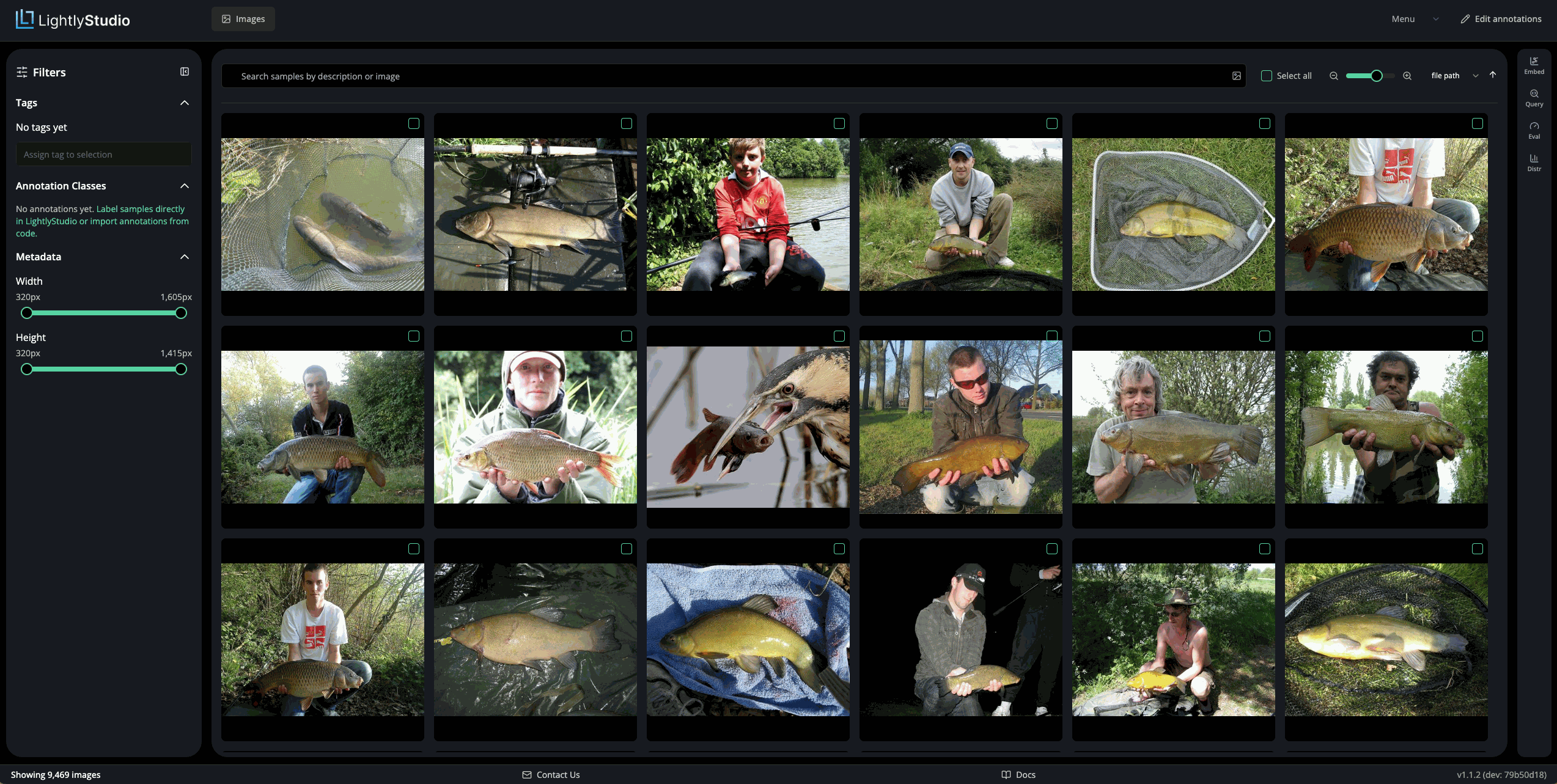
LightlyStudio computes the image embeddings during ingestion, so there is no separate step and no button in the GUI to compute them. The first run also downloads the embedding model, which makes it slower than later runs.

Step 3: Explore the embedding plot

Click Embed in the right-hand tab rail to open the embedding plot. Each point is one image, placed by a two-dimensional projection (PaCMAP) of its embedding. See the embedding plot.

No Embed tab?

The tab only appears when the dataset has embeddings. If it is missing, ingestion ran with embed=False or the embedding model failed to download. Check the output of step 2.

The embedding plot. Each point is one image.

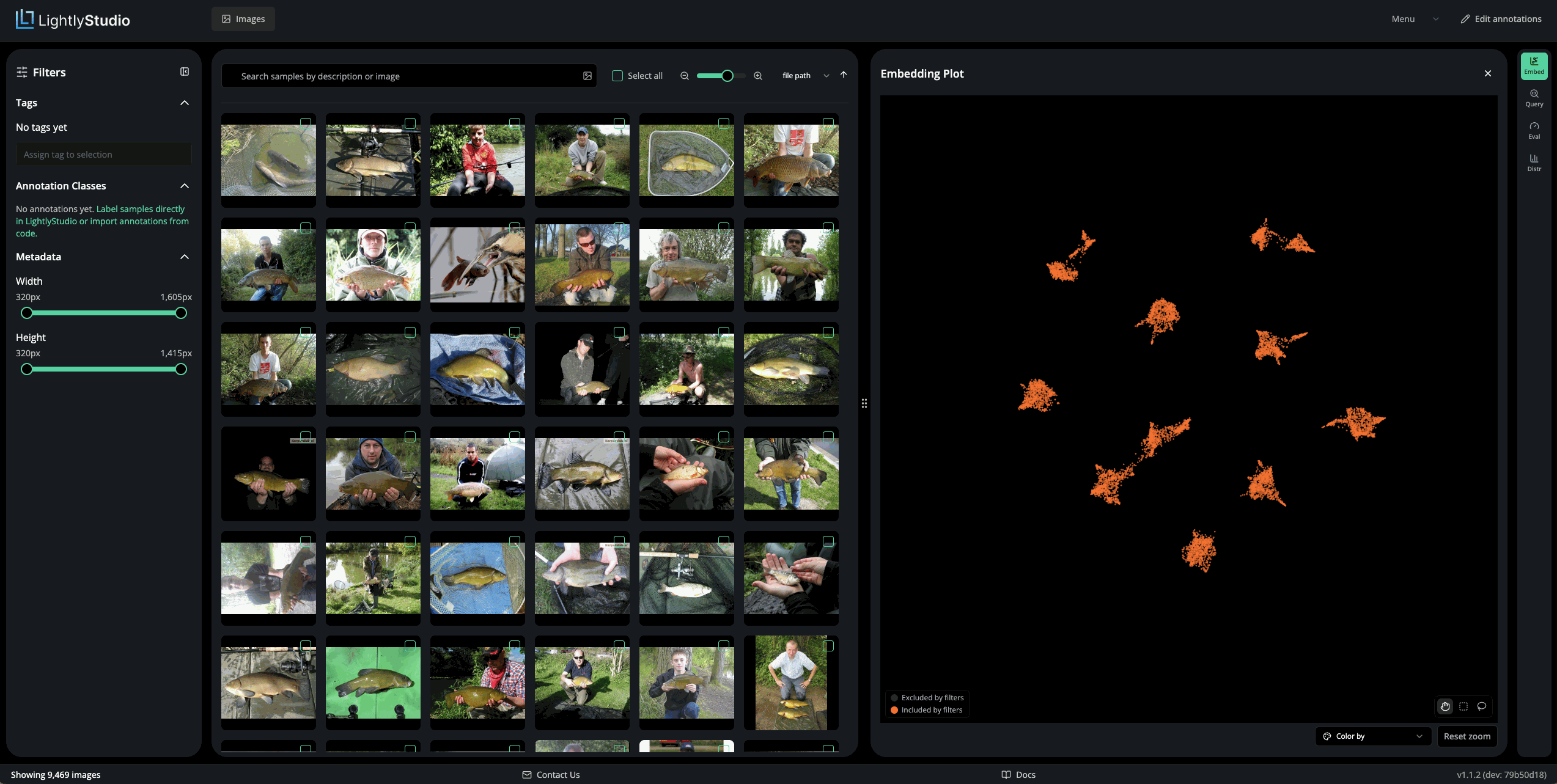
1. Scroll to zoom, and select Pan to drag the view.
2. Hover over several points to preview their images.
3. Look for shared characteristics: object shape, scene type, indoor or outdoor, and background.
4. Compare one group with another elsewhere in the plot.

The projection is approximate. It keeps local neighborhoods, not distances. A visible group is not necessarily one class, and one class can appear in several groups. Treat proximity as a reason to inspect images together, not as proof that they share an annotation class.

To inspect a group together, select it. The plot controls offer Pan , Rectangle , and Lasso . The selected tool stays active after you draw a region. Select Pan to drag the view again. In Pan mode, you can also select with these shortcuts:

Gesture	Result
Shift + drag	Rectangle selection.
Shift + Cmd + drag (Ctrl on Windows)	Freehand lasso selection.

Draw around a small group. On release, the image grid scopes to the samples in that region, and an Embedding Plot Filter entry appears in the sidebar with the count.

A lasso scopes the grid. It does not create annotations, and the plot keeps showing every point, highlighting the ones inside your region.

The recording below shows a hover over golf balls. A rectangle selection then scopes the grid to english springers (a dog breed). A lasso selection scopes it to gas pumps.

Zooming, hovering, and selecting a group in the embedding plot.

Select a region, not everything

A selection that covers every point counts as no filter, and the grid does not change. If nothing happens, your lasso was probably too wide.

Press Esc to clear the selection.

Step 4: Annotate a few reference examples

Choose a few clearly identifiable images from several classes. Parachutes, churches, and garbage trucks are easy to recognize, but use whichever examples you can identify confidently. Lasso a region from step 3 to narrow the grid first, or work from the full grid.

Open an image's detail view. Click Adding to, type my_labels, and select Create: my_labels, or select that source if it already exists. Then use Add classification to assign its annotation class. Put every annotation that you create into this source. Step 8 compares it against the ground truth.

Use these exact annotation class names:

tench              chain_saw    garbage_truck    golf_ball
english_springer   church       gas_pump         parachute
cassette_player    french_horn

The names must match exactly

Step 8 compares annotation classes as text. If you write garbage truck here and the ground truth says garbage_truck, every image of that class counts as a disagreement. Copy the names from this list.

Keep exactly one classification per annotated image in each annotation source. Before assigning a different class, remove the previous classification from that source. Step 8 cannot evaluate an image with multiple classifications in either source.

Annotate two or three clear examples for each class you choose. If you are unsure about an image, consult the class table in step 1, or leave the image for later review.

Add classification in the detail view is the right tool for a few individual images. In step 5 you annotate a whole group of images at once instead.

These examples give you visual references for the groups you review next. This is a manual workflow: reference annotations do not classify their neighbors automatically.

Step 5: Review and annotate a group

The recording shows the whole step: a rectangle selects a group, then Edit annotations applies the church annotation class to all of its images. The new annotation class appears in the sidebar on the left.

Annotating a whole group of images in one action.

Select a group in the embedding plot with the lasso from step 3. Review the images in the scoped grid. Open unclear thumbnails in detail view. Exclude other classes and ambiguous images. Start with a small group so you can inspect every sample.

The images that remain share a class, so you can annotate all of them in one action instead of opening each image.

1. Click Edit annotations in the header, or press E. A panel appears to the right of the grid. Without this step the panel stays hidden.
2. Select the images that belong to the class. Click one image, Shift-click to select a range, or use the Select all checkbox above the grid.
3. In the panel, set Annotation source to my_labels. Type the name to create it if it is not in the list.
4. Set Annotation class to the class of the group. Use the names from step 4.
5. Click Add annotation class and confirm. The panel heading shows how many images are selected, and the dialog repeats the count before you apply.
6. Click Finish Editing when you are done.

Select all follows the current view

Select all selects every image that matches the current view, not only the images on screen. With a lasso region active, that is the region. With no filter, that is all 9,469 images. Check the count in the panel before you apply. You cannot undo the annotations.

Not every group is pure. Deselect the images that do not belong before you apply, or annotate them one at a time in the detail view with Add classification.

Images that already have the class are skipped

Applying a class a second time does not create a second annotation. The message after the run reports how many images changed and how many already had the class.

Open several annotated images again and confirm their classifications before you move on.

Repeat for another group:

1. Press Esc to clear the region.
2. Find another group of similar images and select it in the plot.
3. Review the scoped grid.
4. Annotate the images that belong to the class.

Visual similarity suggests candidates. Your review decides which images get the annotation.

Step 6: Use the legend and restore the view

The plot colored by annotation class.

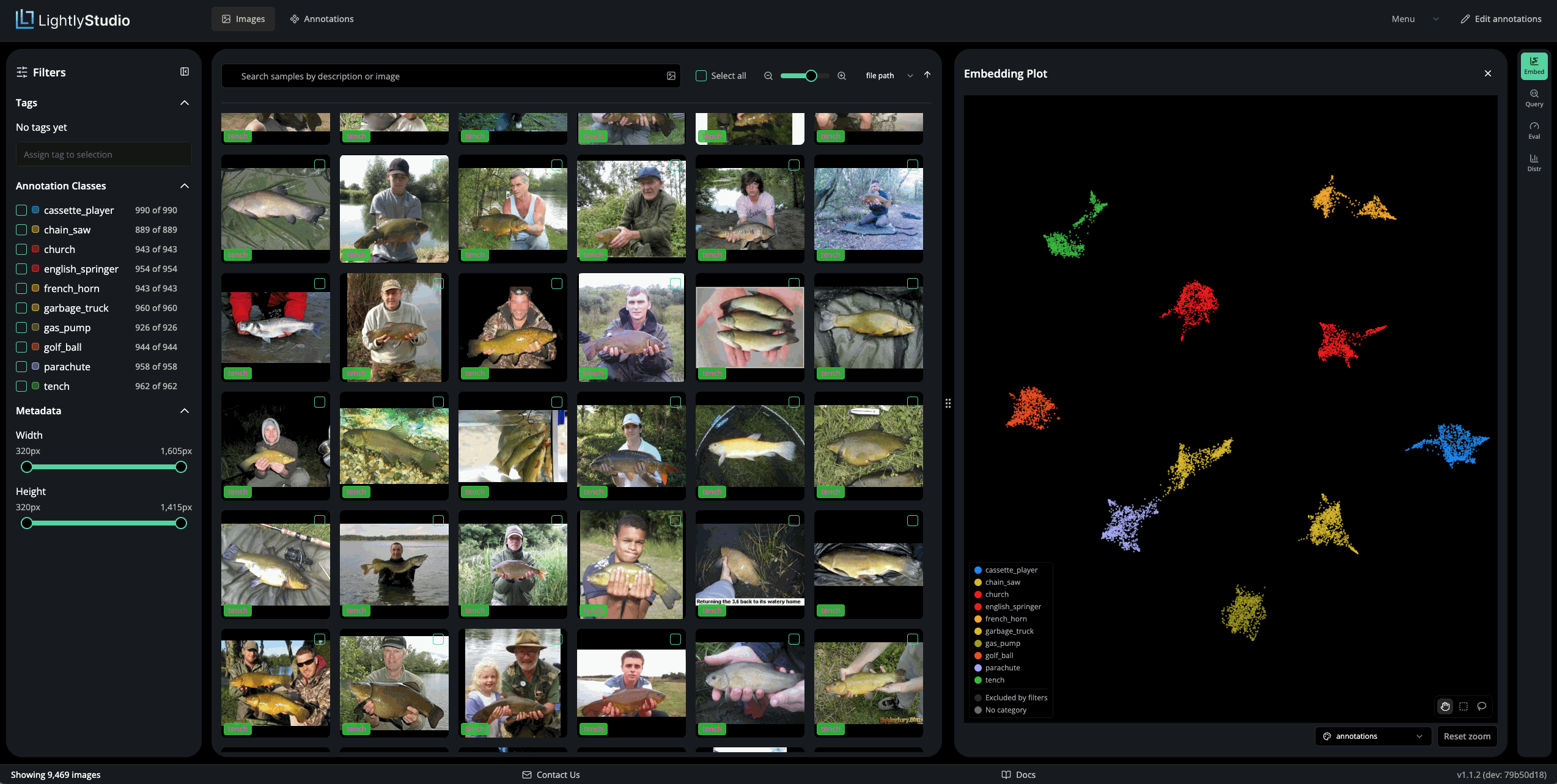
Once you have created annotations, open Color by below the plot and choose annotations. The plot colors each point by its annotation class, and a legend appears in the bottom-left corner.

Control	Try it	Effect
Hover	Hover over a point.	Preview its image.
Legend single-click	Click a class entry, then click it again.	Hide, then show its points.
Legend double-click	Double-click a class entry.	Isolate that class.
Restore classes	Double-click the isolated entry again.	Show the other classes again.
Reset zoom	Click Reset zoom.	Restore the viewport.

The legend also has reserved entries below a divider, such as No category for samples with no annotation. These toggle on a single click, but double-click does not isolate them.

Color by resets the legend

Changing Color by clears which classes you hid, because LightlyStudio reassigns the color slots.

Legend visibility, dataset filters, the lasso region, and the viewport are separate controls. Hiding a class does not delete its images or annotations, and Reset zoom only restores the viewport. To return to an unrestricted view:

1. Press Esc to clear the lasso region.
2. Show any hidden legend entries again.
3. Clear active dataset filters.
4. Click Reset zoom.

Step 7: Load the ground truth

Until now you annotated the images from what you see. Imagenette also ships a reliable class for every image, in its folder names. Load that as a second annotation source, then compare the two.

Stop the GUI with Ctrl+C. Save the following as load_ground_truth.py in the same working directory:

load_ground_truth.py

from pathlib import Path

import lightly_studio as ls
from lightly_studio.core.annotation import CreateClassification

# The folder names of Imagenette are WordNet IDs. These are the annotation class
# names from step 4.
WORDNET_TO_CLASS = {
    "n01440764": "tench",
    "n02102040": "english_springer",
    "n02979186": "cassette_player",
    "n03000684": "chain_saw",
    "n03028079": "church",
    "n03394916": "french_horn",
    "n03417042": "garbage_truck",
    "n03425413": "gas_pump",
    "n03445777": "golf_ball",
    "n03888257": "parachute",
}

dataset = ls.ImageDataset.load(name="imagenette")
for sample in dataset:
    wordnet_id = Path(sample.file_path_abs).parent.name
    sample.add_annotation(
        annotation=CreateClassification(class_name=WORDNET_TO_CLASS[wordnet_id]),
        annotation_source="ground_truth",
    )
print("Ground truth loaded.")

Run it:

python load_ground_truth.py

The script writes one classification for each of the 9,469 images. This takes about one minute. LightlyStudio creates the ten annotation classes when it first reads each name, so there is no separate step for that.

The ground_truth source is separate from your my_labels source. It does not change or overwrite the annotations that you created.

Run this script one time only

add_annotation appends to an annotation source. A second run gives every image a second ground truth annotation, which prevents classification evaluation.

Start the GUI again to see both sources. The Annotation Sources section of the Filters panel on the left now has two checkboxes, my_labels and ground_truth. Select a source to show its annotations, and deselect it to hide them.

With both sources selected, each image you annotated shows annotations from both my_labels and ground_truth. Where your annotation and the ground truth disagree, the two show different annotation classes. The counts under Annotation Classes follow the selection.

Selecting and deselecting annotation sources.

Step 8: Compare your annotations against the ground truth

An evaluation run compares two annotation sources and stores a metric for each image. Save the following as evaluate_imagenette.py in the same working directory:

evaluate_imagenette.py

import lightly_studio as ls

dataset = ls.ImageDataset.load(name="imagenette")
result = dataset.evaluate().classification(
    name="imagenette-review",
    gt_annotation_source="ground_truth",
    pred_annotation_source="my_labels",
)
print(f"Compared {result.sample_count} images.")
ls.start_gui()

Stop the running GUI with Ctrl+C, then run:

python evaluate_imagenette.py

This script uses the ground truth loaded in step 7 without adding annotations. Do not rerun load_ground_truth.py to evaluate your progress.

Each evaluation needs a unique run name within the dataset. Before running this script again, change name to a new value, such as "imagenette-review-2", and select that run in the GUI. Use a new name even if the previous evaluation failed.

An evaluation run uses only the images that are in both annotation sources. Your run therefore covers the images that you annotated, and no others. Images that you did not annotate are skipped. They do not count as errors.

Open the Eval tab in the GUI and select the imagenette-review run:

1. Read the confusion matrix. Green cells on the diagonal are images where you and the ground truth agree.
2. Find the red cells off the diagonal. These are the classes that you and the ground truth assigned differently.
3. Sort the image grid by disagreement to put those images first.
4. Open them in detail view and compare what you see against both annotation classes.

A red cell is not always your error. Some Imagenette images contain more than one of the ten classes. The confusion matrix shows you where visual similarity and annotation class stop agreeing. These are the images that a labeling workflow gets wrong most often.

The recording below opens the confusion matrix and examines three disagreements. The first two images are a french horn, annotated as a golf ball and as a parachute. The third is a gas pump, annotated as a garbage truck. This last image shows a gas pump next to a truck, which explains the disagreement.

Reading the confusion matrix of the imagenette-review run.

For more about evaluation runs and their metrics, see Model Evaluation.

Step 9: Save and export your progress

LightlyStudio persists your annotations in its database. To resume later, rerun explore_imagenette.py from the same working directory. Open an annotated image to verify that its classification is still there. See Reuse Datasets.

To export your classifications:

1. Clear temporary filters and selections, so you export the scope you intend.
2. Open Menu → Export.
3. Choose Image Classifications (CSV) and the my_labels annotation source.
4. Export the file, then check several image paths and their classes against the GUI.

Exporting image classifications from the my_labels annotation source.

Select my_labels and not ground_truth. The ground_truth source is the reference that you loaded in step 7, not the work that you did.

The CSV contains classifications and image paths. It does not package the image files, so keep the original images and the database. Images you have not annotated stay available for later work.

For more export options, see Export.

Conclusion

You imported 9,469 raw images, explored their embeddings, and used groups of similar images to guide labeling. Instead of deciding what every image shows, you reviewed related images together and gave a whole group its shared annotation class in one action. Then you loaded the ground truth of the dataset and measured where your annotations and the ground truth disagree.

Continue with more groups until you reach the coverage you need. After each session, stop the GUI, choose a new run name in evaluate_imagenette.py (for example, "imagenette-review-2"), and rerun it. The confusion matrix shows whether your accuracy holds as you move into groups that are harder to tell apart.

A follow-up workflow could use embeddings and a small set of annotated examples to generate nearest-neighbor suggestions. Keep suggestions in their own annotation source and inspect them before you accept them.

Related guides: Embeddings, which also shows how to load precomputed embeddings instead of computing them at import, Image Dataset, and Annotations.

Edit this page Report an issue Ask in Discord