Advanced Concepts in Self-Supervised Learning

In this section, we will have a look at some more advanced topics around LightlySSL.

Augmentations

Most recent self-supervised learning methods create multiple views of each image during training and learn that embeddings of views from the same image should be as similar as possible. As these views are typically created using augmentations, the model learns to be invariant to certain augmentations.

Different augmentations result in different invariances. The invariances you want to learn heavily depend on the type of downstream task you want to solve. Here, we group the augmentations by the type of invariance they induce and show examples of when such invariances can be useful.

For example, if we use color jittering and random grayscale during the training of a self-supervised model, we train the model to put the two augmented versions of the input image very close to each other in the feature space. We essentially train the model to ignore the color augmentations.

Shape Invariances

Random cropping E.g. We don’t care if an object is small or large or only partially in the image.
Random Horizontal Flip E.g. We don’t care about “left and right” in images.
Random Vertical Flip E.g. We don’t care about “up and down” in images. This can be useful for satellite images.
Random Rotation E.g. We don’t care about the orientation of the camera. This can be useful for satellite images.

Texture Invariances

Gaussian Blur E.g. We don’t care about the details of a person but the overall shape.

Color Invariances

Color Jittering E.g. We don’t care if a car is blue or red
Random Grayscale E.g. We don’t care about the color of a tree
Solarization E.g. We don’t care about color and brightness

Some interesting papers regarding invariances in self-supervised learning:

Note

Picking the right augmentation method seems crucial for the outcome of training models using contrastive learning. For example, if we want to create a model classifying cats by color we should not use strong color augmentations such as color jittering or random grayscale.

Note

Recently, masked image modeling (MIM) has become a popular method for self-supervised learning. MIM is a different approach as the goal is not to map different views of the same image close to each other in the feature space. Instead, the model learns to predict the masked parts of the image. This has the advantage that the model doesn’t learn an invariance with respect to the augmentations. Popular MIM methods are MAE and SimMIM. For a more in-depth discussion of different self-supervised learning methods see A Cookbook of Self-Supervised Learning.

Transforms

LightlySSL uses Torchvision transforms to apply augmentations to images. The LightlySSL transforms module exposes transforms for common self-supervised learning methods.

The most important difference compared to transforms for other tasks, such as classification, object detection, or segmentation, is that self-supervised learning requires multiple views per image. For example, SimCLR uses two views per image while DINO uses two global and multiple, smaller local views per image.

Note

If you use the Command-line tool you have access to all SimCLR augmentations. You find the default parameters here: Default Settings.

Note

Since solarization and random rotations by 90 degrees are not supported in Torchvision, we added them to the transforms module as well.

Custom Transforms

There are three ways how you can customize augmentations in LightlySSL:

Modify the parameters of the transforms provided by LightlySSL:

from lightly.transforms import SimCLRTransform

transform = SimCLRTransform(
    input_size=128,   # resize input images to 128x128 pixels
    cj_prob=0.0,      # disable color jittering
    rr_prob=0.5,      # apply random rotation by 90 degrees with 50% probability
)
Note

You can disable the augmentations by either setting the probability to 0.0 or making sure the augmentation has no effect. For example, random cropping can be disabled by setting min_scale=1.0.

Create a new transform by combining multiple transforms into a MultiViewTransform:

from torchvision import transforms as T
from lightly.transforms.multi_view_transform import MultiViewTransform

# Create a global view transform that crops 224x224 patches from the input image.
global_view = T.Compose([
    T.RandomResizedCrop(size=224, scale=(0.08, 1.0)),
    T.RandomHorizontalFlip(p=0.5),
    T.RandomGrayscale(p=0.5),
    T.ToTensor(),
])

# Create a local view transform that crops a random portion of the input image and resizes it to a 96x96 patch.
local_view = T.Compose([
    T.RandomResizedCrop(size=96, scale=(0.05, 0.4)),
    T.RandomHorizontalFlip(p=0.5),
    T.RandomGrayscale(p=0.5),
    T.ToTensor(),
])

# Combine the transforms. Every transform will create one view.
# The final transform will create four views: two global and two local views.
transform = MultiViewTransform([global_view, global_view, local_view, local_view])
views = transform(image)

Write a completely new Torchvision transform. One of the benefits of Lightly is that it doesn’t restrict you to a specific framework. If you need a special transform then you can write it yourself. Just make sure to adapt your training loop if required:

from torch.utils.data import DataLoader

class MyTransform:
    def __call__(self, image):
        # Overwrite this method and apply custom augmentations to your image.

transform = MyTransform(...)
dataset = LightlyDataset(..., transform=transform)
dataloader = DataLoader(dataset, ...)
for batch in dataloader:
    views = ... # get views from the batch, this depends on your transform

Previewing Augmentations

Note

This section is outdated and still uses the old collate functions which are deprecated since v1.4.0. We will update this section soon.

It often can be very useful to understand how the image augmentations we pick affect the input dataset. We provide a few helper methods that make it very easy to preview augmentations using LightlySSL.

import glob

from PIL import Image

import lightly

# let's get all jpg filenames from a folder
glob_to_data = "/datasets/clothing-dataset/images/*.jpg"
fnames = glob.glob(glob_to_data)

# load the first two images using pillow
input_images = [Image.open(fname) for fname in fnames[:2]]

# create our colalte function
collate_fn_simclr = lightly.data.SimCLRCollateFunction()

# plot the images
fig = lightly.utils.debug.plot_augmented_images(input_images, collate_fn_simclr)

# let's disable blur
collate_fn_simclr_no_blur = lightly.data.SimCLRCollateFunction()
fig = lightly.utils.debug.plot_augmented_images(input_images, collate_fn_simclr_no_blur)

# we can also use the DINO collate function instead
collate_fn_dino = lightly.data.DINOCollateFunction()
fig = lightly.utils.debug.plot_augmented_images(input_images, collate_fn_dino)

You can run the code in a Jupyter Notebook to quickly explore the augmentations. Once you run plot_augmented_images you should see the original images as well as their augmentations next to them.

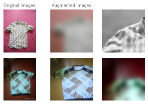
Example augmentations of the SimCLRCollateFunction function on images from the clothing dataset.

The images seem rather blurry! However, we don’t want our model to ignore small details. Let’s disable Gaussian Blur and check again:

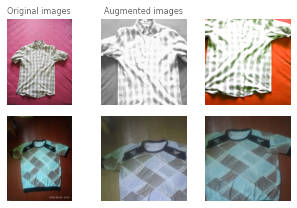
Example augmentations of the SimCLRCollateFunction function on images from the clothing dataset.

We can also repeat the experiment for the DINOCollateFunction to see what our DINO model would see during training.

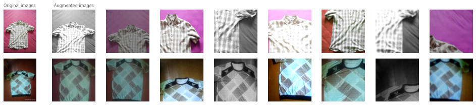
Example augmentations of the DINOCollateFunction function on images from the clothing dataset.

Models

See the Models section for a list of models that are available in LightlySSL.

Do you know a model that should be on this list? Please add an issue on GitHub :)

All models have a backbone component. This could be a ResNet, Vision Transformer, or any other vision model. When creating a self-supervised learning model you pass it a backbone. You need to make sure the backbone output dimension matches the input dimension of the head component for the respective self-supervised model.

LightlySSL has a built-in generator for ResNets. However, the model architecture slightly differs from the official ResNet implementation. The difference is in the first few layers. Whereas the official ResNet starts with a 7x7 convolution the one from LightlySSL has a 3x3 convolution.

The 3x3 convolution variant is more efficient (fewer parameters and faster processing) and is better suited for small input images (32x32 pixels or 64x64 pixels). We recommend using the LightlySSL variant for cifar10 or running the model on a microcontroller (see https://github.com/ARM-software/EndpointAI/tree/master/ProofOfConcepts/Vision/OpenMvMaskDefaults)
However, the 7x7 convolution variant is better suited for larger images since the number of features is smaller due to the stride and additional MaxPool2d layer. For benchmarking against other academic papers on datasets such as ImageNet, Pascal VOC, MOCO, etc. use the Torchvision variant.

from torch import nn

# Create a Lightly\ **SSL** ResNet.
from lightly.models import ResNetGenerator
resnet = ResNetGenerator('resnet-18')
# Ignore the classification layer as we want the features as output.
resnet.linear = nn.Identity()

# Alternatively create a Torchvision ResNet backbone.
import torchvision
resnet_torchvision = torchvision.models.resnet18()
# Ignore the classification layer as we want the features as output.
resnet_torchvision.fc = nn.Identity()

# Create a SimCLR model based on ResNet.
class SimCLR(torch.nn.Module):
    def __init__(self, backbone, hidden_dim, out_dim):
        super().__init__()
        self.backbone = backbone
        self.projection_head = SimCLRProjectionHead(hidden_dim, hidden_dim, out_dim)

    def forward(self, x):
        h = self.backbone(x).flatten(start_dim=1)
        z = self.projection_head(h)
        return z

resnet_simclr = SimCLR(backbone, hidden_dim=512, out_dim=128)

You can also use custom backbones with LightlySSL. We provide a colab notebook to show how you can use torchvision or timm models.

Losses

We provide the most common loss functions for self-supervised learning in the loss module.

Memory Bank

Since contrastive learning methods benefit from many negative examples, larger batch sizes are preferred. However, not everyone has a multi GPU cluster at hand. Therefore, alternative tricks and methods have been derived in research. One of them is a memory bank keeping past examples as additional negatives.

For an example of the memory bank in action have a look at Tutorial 2: Train MoCo on CIFAR-10.

For more information check the documentation: lightly.loss.memory_bank.MemoryBankModule.

# to create a NTXentLoss with a memory bank (like for MoCo) set the
# memory_bank_size parameter to a value > 0 and specify the feature dimension
from lightly.loss import NTXentLoss
criterion = NTXentLoss(memory_bank_size=(4096, 128))
# the memory bank is used automatically for every forward pass
y0, y1 = resnet_moco(x0, x1)
loss = criterion(y0, y1)

Obtaining Good Embeddings

We optimize the workflow of selecting only important datapoints by using low-dimensional embeddings. This has two benefits:

Low-dimensional embeddings have more meaningful distance metrics. We know that the data usually lies on a manifold in high-dimensional spaces (see curse of dimensionality). Even very similar samples might have a high L2-distance or low cosine similarity in high embeddings.
Most algorithms to select a subset based on the embeddings scale with the dimensionality. Therefore low-dimensional embeddings can significantly reduce computing time.

We leverage self-supervised learning to obtain good features/representations/embedddings of your unlabeled data. The quality of the representations depends heavily on the chosen augmentations. For example, imagine you want to train a classifier to detect healthy and unhealthy leaves. Training self-supervised models with color augmentation enabled would make the model and therefore the embeddings invariant towards different colors. However, the color might be a very important feature of the leave to determine whether it is healthy (green) or not (brown).

Monitoring Embedding Quality

We provide several tools to assess the embedding quality during model training. The Benchmark Module runs a KNN benchmark on a validation set after every training epoch. Measuring KNN accuracy during training is an efficient way to monitor model training and does not require expensive fine-tuning.

We also provide a helper function to monitor representation collapse. Representation collapse can happen during unstable training and results in the model predicting the same, or very similar, representations for all images. This is of course disastrous for model training as we want to the representations to be as different as possible between images! The std_of_l2_normalized helper function can be used on any representations as follows:

from lightly.utils.debug import std_of_l2_normalized
representations = model(images)
std_of_l2_normalized(representations)

A value close to 0 indicates that the representations have collapsed. A value close to 1/sqrt(dimensions), where dimensions are the number of representation dimensions, indicates that the representations are stable. Below we show model training outputs from a run where the representations collapse and one where they don’t collapse.

# run with collapse
epoch: 00, loss: -0.78153, representation std: 0.02611
epoch: 01, loss: -0.96428, representation std: 0.02477
epoch: 02, loss: -0.97460, representation std: 0.01636
epoch: 03, loss: -0.97894, representation std: 0.01936
epoch: 04, loss: -0.97770, representation std: 0.01565
epoch: 05, loss: -0.98308, representation std: 0.01192
epoch: 06, loss: -0.98641, representation std: 0.01133
epoch: 07, loss: -0.98673, representation std: 0.01583
epoch: 08, loss: -0.98708, representation std: 0.01146
epoch: 09, loss: -0.98654, representation std: 0.01656

# run without collapse
epoch: 00, loss: -0.35693, representation std: 0.06708
epoch: 01, loss: -0.69948, representation std: 0.05853
epoch: 02, loss: -0.74144, representation std: 0.05710
epoch: 03, loss: -0.74297, representation std: 0.05804
epoch: 04, loss: -0.71997, representation std: 0.06441
epoch: 05, loss: -0.70027, representation std: 0.06738
epoch: 06, loss: -0.70543, representation std: 0.06898
epoch: 07, loss: -0.71539, representation std: 0.06875
epoch: 08, loss: -0.72629, representation std: 0.06991
epoch: 09, loss: -0.72912, representation std: 0.06945

We note that in both runs the loss decreases, indicating that the model is making progress. The representation std shows, however, that the two runs are very different. The std in the first run decreases towards zero which means that the representations become more and more similar. The std in the second run remains stable and close to the expected value of 1/sqrt(dimensions) = 0.088 for this run (dimensions = 128). If we had only monitored the loss, we would not have noticed the representation collapse in the first run and continued training, using up valuable time and compute resources.