Train a World Model and Plan with It

A world model predicts what an agent will see after it does an action. In this tutorial, we train LeWM from LeWorldModel and use it to move an agent to a goal.

LeWM learns from frames and actions only. It does not use rewards or labels. An encoder turns each frame into an embedding. A predictor predicts the embedding of the next frame from the current embedding and the action. The SIGReg term of the loss prevents the collapse of all embeddings to one point.

The environment is a small room with a wall. We write it in this tutorial, so there is no dataset to download. Training takes about 5 minutes on one GPU.

In this tutorial you will learn:

• How to collect episodes from an environment

• How to train LeWM with lightly

• How to make sure that the model uses the actions

• How to read the predictions with a probe and a decoder

• How to plan with the model to reach a goal

Imports

This tutorial needs timm for the encoder and matplotlib for the plots.

pip install "lightly[timm]" matplotlib

import copy
import math

import matplotlib.pyplot as plt
import numpy as np
import timm
import torch
from matplotlib.patches import Rectangle
from torch import nn
from torch.utils.data import DataLoader, TensorDataset

from lightly.loss import LeWMLoss
from lightly.models.modules import (
    ActionEncoder,
    LatentDynamicsPredictor,
    LeWMProjectionHead,
)

Configuration

The default configuration trains for 10 epochs on 1000 episodes. Training needs about 2 GB of GPU memory. On a CPU, use fewer episodes and epochs to make the run shorter.

seed = 0
num_episodes = 1000
episode_length = 32
clip_length = 4
batch_size = 128
epochs = 10
embed_dim = 192

if torch.cuda.is_available():
    device = "cuda"
elif torch.backends.mps.is_available():
    device = "mps"
else:
    device = "cpu"

torch.manual_seed(seed)
rng = np.random.default_rng(seed)

The environment

The environment is a room of 64x64 pixels. A vertical wall divides the room in two halves, and the agent can only go through the door in the wall. The state is the position of the top-left corner of the agent. An action is a vector (dx, dy) in [-1, 1]. It moves the agent by up to 6 pixels on each axis. The agent stops when it touches the wall or the border.

class WallWorld:
    size = 64  # Width and height of a frame in pixels.
    agent = 8  # Side length of the square agent.
    wall = (30.0, 34.0)  # Columns of the wall.
    door = (24.0, 40.0)  # Rows of the door in the wall.
    max_step = 6.0  # Largest movement on each axis in one step.

    def blocked(self, pos):
        x, y = pos
        in_wall_columns = x < self.wall[1] and x + self.agent > self.wall[0]
        in_door_rows = y >= self.door[0] and y + self.agent <= self.door[1]
        return in_wall_columns and not in_door_rows

    def random_position(self, rng):
        while True:
            pos = rng.uniform(0, self.size - self.agent, size=2)
            if not self.blocked(pos):
                return pos

    def step(self, pos, action):
        # Move along x, then along y. Stop at the wall on each axis.
        delta = np.clip(action, -1, 1) * self.max_step
        pos = np.array(pos, dtype=np.float64)
        pos[0] = np.clip(pos[0] + delta[0], 0, self.size - self.agent)
        if self.blocked(pos):
            pos[0] = self.wall[0] - self.agent if delta[0] > 0 else self.wall[1]
        pos[1] = np.clip(pos[1] + delta[1], 0, self.size - self.agent)
        if self.blocked(pos):
            pos[1] = self.door[1] - self.agent if delta[1] > 0 else self.door[0]
        return pos

    def render(self, positions):
        # Draw frames with shape (..., 3, 64, 64) for positions (..., 2).
        centers = np.arange(self.size) + 0.5
        x = positions[..., 0, None, None]
        y = positions[..., 1, None, None]
        agent = (centers[None, :] >= x) & (centers[None, :] < x + self.agent)
        agent = agent & (centers[:, None] >= y) & (centers[:, None] < y + self.agent)
        wall = (centers >= self.wall[0]) & (centers < self.wall[1])
        door = (centers >= self.door[0]) & (centers < self.door[1])
        wall = wall[None, :] & ~door[:, None]
        background = (0.08, 0.08, 0.12)
        wall_color = (0.55, 0.55, 0.6)
        agent_color = (1.0, 0.6, 0.1)
        frames = np.empty(positions.shape[:-1] + (3, self.size, self.size), np.float32)
        for c in range(3):
            frames[..., c, :, :] = np.where(
                agent, agent_color[c], np.where(wall, wall_color[c], background[c])
            )
        return frames


world = WallWorld()

Collect episodes

LeWM learns from recorded episodes. It does not need a good policy, so we use a random one. The policy keeps its last action with a probability of 0.8. As a result, the agent moves in straight lines for some steps and often goes through the door.

def collect(num_episodes, num_steps, rng, keep_prob=0.8):
    positions = np.empty((num_episodes, num_steps + 1, 2), np.float32)
    actions = np.empty((num_episodes, num_steps, 2), np.float32)
    for episode in range(num_episodes):
        pos = world.random_position(rng)
        action = rng.uniform(-1, 1, size=2)
        positions[episode, 0] = pos
        for t in range(num_steps):
            if rng.random() > keep_prob:
                action = rng.uniform(-1, 1, size=2)
            pos = world.step(pos=pos, action=action)
            actions[episode, t] = action
            positions[episode, t + 1] = pos
    return positions, actions


train_positions, train_actions = collect(
    num_episodes=num_episodes, num_steps=episode_length, rng=rng
)
test_positions, test_actions = collect(
    num_episodes=64, num_steps=episode_length, rng=rng
)

The plot shows one of the episodes. The agent slides along the wall and then goes through the door.

wall_center = sum(world.wall) / 2
left = train_positions[..., 0] + world.agent / 2 < wall_center
crossing = np.argmax(left.any(axis=1) & ~left.all(axis=1))  # 0 if none crosses
frames = world.render(train_positions[crossing, ::4])
fig, axes = plt.subplots(1, len(frames), figsize=(2 * len(frames), 2.4))
for t, (ax, frame) in enumerate(zip(axes, frames)):
    ax.imshow(frame.transpose(1, 2, 0))
    ax.set_title(f"step {4 * t}")
    ax.axis("off")
plt.show()

The training data are clips of clip_length consecutive frames and the actions between them. Each episode gives 30 clips that overlap. We store only the positions and draw the frames when we need them.

clip_starts = range(episode_length + 2 - clip_length)
clip_positions = np.concatenate(
    [train_positions[:, s : s + clip_length] for s in clip_starts]
)
clip_actions = np.concatenate(
    [train_actions[:, s : s + clip_length - 1] for s in clip_starts]
)
dataset = TensorDataset(
    torch.from_numpy(clip_positions), torch.from_numpy(clip_actions)
)
dataloader = DataLoader(dataset, batch_size=batch_size, shuffle=True, drop_last=True)

The model

LeWM has four parts:

• The encoder is a ViT-tiny from timm. It turns a frame into a vector of 192 numbers.

• The projection head maps this vector to the embedding.

• The action encoder maps an action to a vector with the width of the embedding.

• The predictor is a causal transformer. It predicts the embedding of the next frame from the embeddings and the actions so far.

The predictor sees at most 3 frames, which is the context of the training clips.

class LeWM(nn.Module):
    def __init__(self, embed_dim, history):
        super().__init__()
        self.backbone = timm.create_model(
            "vit_tiny_patch16_224",
            pretrained=False,
            img_size=64,
            num_classes=0,
            dynamic_img_size=True,
        )
        self.projection_head = LeWMProjectionHead(
            input_dim=self.backbone.num_features, output_dim=embed_dim
        )
        self.action_encoder = ActionEncoder(action_dim=2, output_dim=embed_dim)
        self.predictor = LatentDynamicsPredictor(
            num_frames=history,
            input_dim=embed_dim,
            hidden_dim=384,
            depth=4,
            num_heads=6,
        )

    def encode(self, frames):
        # Encode frames (B, T, 3, H, W) to embeddings (B, T, D).
        batch_size, num_frames = frames.shape[:2]
        features = self.backbone(frames.flatten(0, 1))
        embeddings = self.projection_head(features)
        return embeddings.unflatten(0, (batch_size, num_frames))

    def predict(self, embeddings, actions):
        # Predict the next embedding for every frame (B, T, D).
        return self.predictor(embeddings, action_emb=self.action_encoder(actions))


model = LeWM(embed_dim=embed_dim, history=clip_length - 1).to(device)

Train the model

For each clip, the predictor gets the embeddings of frames 1 to 3 and the three actions. It predicts the embeddings of frames 2 to 4. lightly.loss.LeWMLoss adds two terms. The prediction term is the mean squared error between the predicted and the real embeddings. The SIGReg term pushes the distribution of the embeddings to a standard Gaussian, so that the encoder cannot map all frames to one point.

criterion = LeWMLoss(lambda_param=0.1).to(device)  # Moves the SIGReg buffers.
optimizer = torch.optim.AdamW(model.parameters(), lr=3e-4, weight_decay=0.05)
total_steps = epochs * len(dataloader)
warmup_steps = max(1, total_steps // 20)
scheduler = torch.optim.lr_scheduler.LambdaLR(
    optimizer,
    lambda step: min(1.0, (step + 1) / warmup_steps)
    * 0.5
    * (1 + math.cos(math.pi * step / total_steps)),
)

history = []
for epoch in range(epochs):
    model.train()
    term_sums = torch.zeros(2, device=device)
    for positions, actions in dataloader:
        frames = torch.from_numpy(world.render(positions.numpy())).to(device)
        actions = actions.to(device)
        embeddings = model.encode(frames)
        predicted = model.predict(embeddings[:, :-1], actions)
        loss = criterion(
            predicted=predicted, target=embeddings[:, 1:], embeddings=embeddings
        )
        optimizer.zero_grad()
        loss.backward()
        optimizer.step()
        scheduler.step()
        # Log both terms for the plot. SIGReg expects the batch in dimension -2.
        with torch.no_grad():
            embeddings = embeddings.detach()
            prediction = (predicted - embeddings[:, 1:]).square().mean()
            sigreg = criterion.sigreg(embeddings.transpose(0, 1))
            term_sums += torch.stack([prediction, sigreg])
    history.append((term_sums / len(dataloader)).tolist())
    print(
        f"epoch {epoch}: prediction {history[-1][0]:.4f}, SIGReg {history[-1][1]:.3f}"
    )

fig, axes = plt.subplots(1, 2, figsize=(10, 3.5))
for ax, values, title in zip(axes, zip(*history), ["prediction term", "SIGReg term"]):
    ax.plot(range(1, epochs + 1), values, marker="o")
    ax.set_xlabel("epoch")
    ax.set_title(title)
fig.tight_layout()
plt.show()

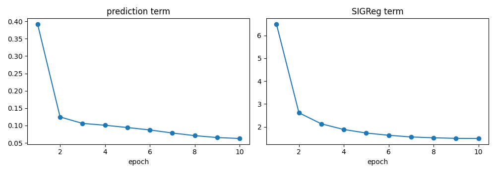
epoch 0: prediction 0.3918, SIGReg 6.490
epoch 1: prediction 0.1246, SIGReg 2.615
epoch 2: prediction 0.1061, SIGReg 2.131
epoch 3: prediction 0.1008, SIGReg 1.885
epoch 4: prediction 0.0941, SIGReg 1.730
epoch 5: prediction 0.0872, SIGReg 1.631
epoch 6: prediction 0.0784, SIGReg 1.558
epoch 7: prediction 0.0708, SIGReg 1.522
epoch 8: prediction 0.0653, SIGReg 1.497
epoch 9: prediction 0.0626, SIGReg 1.491

Check the batch norm

The projection head has a batch norm layer. In training mode, it uses the statistics of the batch. In eval mode, it uses running statistics. We plan in eval mode, so the two modes must give almost the same embeddings. We compare them on a batch of test frames. A copy of the head runs in training mode, so that the running statistics do not change.

model.eval()
with torch.no_grad():
    frames = torch.from_numpy(world.render(test_positions[:, 0])).to(device)
    features = model.backbone(frames)
    eval_embeddings = model.projection_head(features)
    train_embeddings = copy.deepcopy(model.projection_head).train()(features)
    gap = (train_embeddings - eval_embeddings).square().mean()
    gap = gap / eval_embeddings.var(dim=0).mean()
print(f"difference between train and eval mode: {gap:.3f} of the variance")

difference between train and eval mode: 0.052 of the variance

Does the model use the actions?

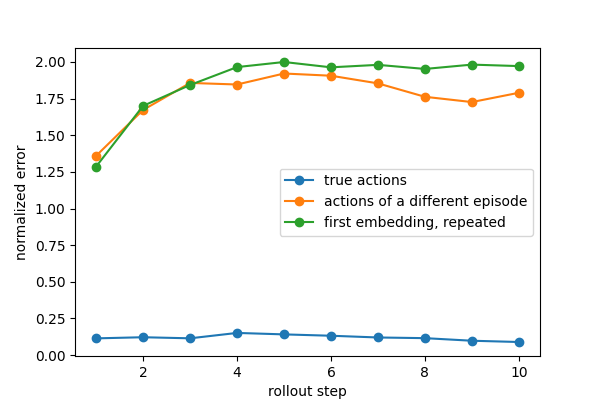
A low prediction loss does not prove that the model uses the actions. In many environments, the motion in the past frames predicts most of the next frame. To make sure that the model uses the actions, we do rollouts on test episodes. A rollout starts from the embedding of one frame. The predictor predicts the next embedding and then uses this prediction as its next input.

We compare three rollouts of 10 steps:

• with the true actions of the episode

• with the actions of a different episode

• without the model: the embedding of the first frame, repeated

The plot shows the mean squared error to the real embeddings, divided by the variance of the embeddings. A model that uses the actions has a much lower error with the true actions.

@torch.no_grad()
def encode_positions(positions, chunk_size=512):
    # Draw and encode frames for positions (..., 2). Returns (..., D) on the CPU.
    flat = positions.reshape(-1, 2)
    embeddings = []
    for i in range(0, len(flat), chunk_size):
        frames = torch.from_numpy(world.render(flat[i : i + chunk_size])).to(device)
        embeddings.append(model.encode(frames[None])[0].cpu())
    return torch.cat(embeddings).reshape(*positions.shape[:-1], -1)


@torch.no_grad()
def rollout(context, actions):
    # Predict one embedding per action. context: (B, 1, D), actions: (B, H, 2).
    action_emb = model.action_encoder(actions)
    return model.predictor.rollout(
        context, action_emb=action_emb, steps=actions.shape[1]
    )


horizon = 10
test_embeddings = encode_positions(test_positions).to(device)
test_actions_t = torch.from_numpy(test_actions).to(device)
context = test_embeddings[:, :1]
target = test_embeddings[:, 1 : horizon + 1]
variance = target.var(dim=(0, 1)).mean()
rollouts = {
    "true actions": rollout(context=context, actions=test_actions_t[:, :horizon]),
    "actions of a different episode": rollout(
        context=context, actions=test_actions_t[:, :horizon].roll(1, dims=0)
    ),
    "first embedding, repeated": context.expand_as(target),
}
plt.figure(figsize=(6, 4))
for label, predicted in rollouts.items():
    error = (predicted - target).square().mean(dim=(0, 2)) / variance
    plt.plot(range(1, horizon + 1), error.cpu(), marker="o", label=label)
plt.xlabel("rollout step")
plt.ylabel("normalized error")
plt.legend()
plt.show()

Read the predictions with a probe

An embedding is a vector of 192 numbers, and we do not know what each number means. A probe is a small model that reads one property from the embedding, here the position of the agent. We know the position for every frame because we made the frames. Thus, we can train the probe with this position as the target. The probe is not part of the world model. We train it after the world model, and the encoder does not change.

The LeWM paper uses linear probes and MLP probes. Here, we use an MLP with one hidden layer, because it reads the position more exactly. If the probe gives the position of new frames with a small error, the embedding contains the position.

probe_positions = train_positions[:200].reshape(-1, 2)
probe_embeddings = encode_positions(probe_positions)
probe_targets = torch.from_numpy(probe_positions) / world.size
probe = nn.Sequential(nn.Linear(embed_dim, 256), nn.ReLU(), nn.Linear(256, 2))
probe_optimizer = torch.optim.Adam(probe.parameters(), lr=1e-3)
for step in range(2000):
    loss = (probe(probe_embeddings) - probe_targets).square().mean()
    probe_optimizer.zero_grad()
    loss.backward()
    probe_optimizer.step()


@torch.no_grad()
def read_position(embeddings):
    # Apply the probe to embeddings (..., D). Returns positions (..., 2) in pixels.
    return probe(embeddings.cpu()) * world.size


error = read_position(test_embeddings) - torch.from_numpy(test_positions)
print(f"probe error on test frames: {error.norm(dim=-1).mean():.1f} pixels")

probe error on test frames: 0.6 pixels

Now we apply the same probe to the embeddings of a rollout. These embeddings come from the predictor, not from a frame. Thus, the probe shows where the model expects the agent to be.

imagined = read_position(rollouts["true actions"])
error = imagined - torch.from_numpy(test_positions[:, 1 : horizon + 1])
print(f"probe error on predicted embeddings: {error.norm(dim=-1).mean():.1f} pixels")

probe error on predicted embeddings: 2.5 pixels

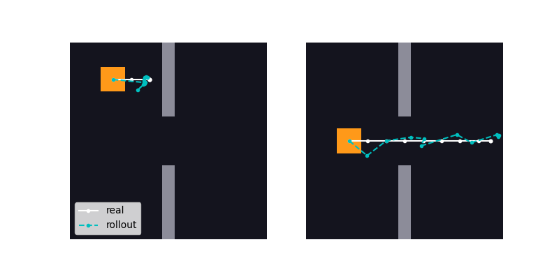
The wall is a good test for the model. In the plot, the agent moves right for 10 steps from two start positions. On the left, the wall blocks the agent. On the right, the agent goes through the door. The dashed line is the rollout, read with the probe.

def push_right(starts, num_steps=10):
    actions = np.tile(np.float32([1.0, 0.0]), (len(starts), num_steps, 1))
    real = [starts]
    for t in range(num_steps):
        real.append(
            np.stack(
                [world.step(pos=p, action=a) for p, a in zip(real[-1], actions[:, t])]
            )
        )
    context = encode_positions(starts[:, None]).to(device)
    predicted = rollout(context=context, actions=torch.from_numpy(actions).to(device))
    real = np.stack(real, axis=1)
    imagined = read_position(predicted).numpy()
    imagined = np.concatenate([starts[:, None], imagined], axis=1)
    return real, imagined


real, imagined = push_right(np.array([[10.0, 8.0], [10.0, 28.0]]))
fig, axes = plt.subplots(1, 2, figsize=(8, 4))
for ax, real_path, imagined_path in zip(axes, real, imagined):
    ax.imshow(world.render(real_path[0]).transpose(1, 2, 0), extent=(0, 64, 64, 0))
    center = world.agent / 2
    ax.plot(*(real_path + center).T, "w-o", markersize=3, label="real")
    ax.plot(*(imagined_path + center).T, "c--o", markersize=3, label="rollout")
    ax.axis("off")
axes[0].legend(loc="lower left")
plt.show()

The same test with 200 random start positions in the left half of the room shows how often the rollout agrees with the environment on one question: does the agent get through the wall?

starts = np.stack([rng.uniform(0, 22, 200), rng.uniform(0, 56, 200)], axis=1)
real, imagined = push_right(starts)
through_real = real[:, -1, 0] + world.agent / 2 > wall_center
through_imagined = imagined[:, -1, 0] + world.agent / 2 > wall_center
print(
    f"agreement with the environment: {np.mean(through_real == through_imagined):.0%}"
)

agreement with the environment: 96%

Look at the predictions with a decoder

A decoder turns an embedding back into a frame. LeWM does not need a decoder, and the decoder does not change the world model. We train it after the world model, on frozen embeddings, only to look at the predictions.

class FrameDecoder(nn.Module):
    def __init__(self, embed_dim):
        super().__init__()
        self.project = nn.Linear(embed_dim, 512 * 4 * 4)
        layers = []
        for in_channels, out_channels in [(512, 256), (256, 128), (128, 64), (64, 64)]:
            layers += [
                nn.Upsample(scale_factor=2),
                nn.Conv2d(in_channels, out_channels, kernel_size=3, padding=1),
                nn.GroupNorm(32, out_channels),
                nn.SiLU(),
            ]
        layers += [nn.Conv2d(64, 3, kernel_size=3, padding=1), nn.Sigmoid()]
        self.layers = nn.Sequential(*layers)

    def forward(self, embeddings):
        return self.layers(self.project(embeddings).view(-1, 512, 4, 4))


decoder = FrameDecoder(embed_dim).to(device)
decoder_optimizer = torch.optim.AdamW(decoder.parameters(), lr=1e-3)
decoder_positions = train_positions.reshape(-1, 2)
decoder_embeddings = encode_positions(decoder_positions)
for step in range(1000):
    index = rng.integers(0, len(decoder_positions), 256)
    frames = torch.from_numpy(world.render(decoder_positions[index])).to(device)
    reconstructed = decoder(decoder_embeddings[index].to(device))
    loss = nn.functional.mse_loss(reconstructed, frames)
    decoder_optimizer.zero_grad()
    loss.backward()
    decoder_optimizer.step()
print(f"decoder error: {loss.item():.5f}")

decoder error: 0.00005

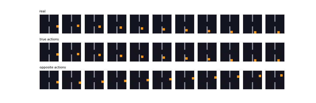
The first row shows a test episode. The second row decodes a rollout with the true actions. The third row decodes a rollout with the opposite actions. All rows start from the same frame.

opposite = rollout(context=context[:1], actions=-test_actions_t[:1, :horizon])
with torch.no_grad():
    first = torch.from_numpy(world.render(test_positions[0, :1])).to(device)
    rows = {
        "real": torch.from_numpy(world.render(test_positions[0, : horizon + 1])),
        "true actions": torch.cat([first, decoder(rollouts["true actions"][0])]),
        "opposite actions": torch.cat([first, decoder(opposite[0])]),
    }
fig, axes = plt.subplots(3, horizon + 1, figsize=(horizon + 1, 3.6))
for row, (label, frames) in enumerate(rows.items()):
    for t in range(horizon + 1):
        axes[row, t].imshow(frames[t].cpu().numpy().transpose(1, 2, 0).clip(0, 1))
        axes[row, t].axis("off")
    axes[row, 0].set_title(label, fontsize=8, loc="left")
plt.show()

Plan with the model

Planning uses the model to select actions. The planner gets the current frame and a goal frame. It tries many action sequences in the model and keeps the sequence whose predicted embeddings are nearest to the embedding of the goal frame. The model does not change during planning.

We use the cross-entropy method (CEM). A plan is a sequence of 8 actions. CEM keeps a Gaussian distribution over plans: mean is the best plan so far, and std is the range around it that CEM still tries. Each iteration does these steps:

1. Sample 300 plans from the distribution.

2. Do a rollout for each plan from the current embedding.

3. Calculate the cost of each plan: the mean squared distance between the predicted embeddings and the goal embedding, averaged over the 8 steps.

4. Set mean and std to the mean and standard deviation of the 30 plans with the lowest cost.

After 10 iterations, mean is the plan. plan makes plans for many episodes at the same time, so every tensor has a batch dimension B.

Note

The LeWM paper uses the distance at the last step of the plan only. The average over all steps makes the agent go to the goal early and stay there. On this environment, it gives a much higher success rate.

plan_horizon = 8


@torch.no_grad()
def plan(
    current, goal, horizon=plan_horizon, num_samples=300, num_iters=10, num_elites=30
):
    # current, goal: embeddings (B, D). Returns plans (B, horizon, 2).
    batch, dim = current.shape
    mean = torch.zeros(batch, horizon, 2, device=device)
    std = torch.ones(batch, horizon, 2, device=device)
    context = current.repeat_interleave(num_samples, dim=0).unsqueeze(1)
    for _ in range(num_iters):
        noise = torch.randn(batch, num_samples, horizon, 2, device=device)
        candidates = (mean[:, None] + std[:, None] * noise).clamp(-1, 1)
        predicted = rollout(context=context, actions=candidates.flatten(0, 1))
        predicted = predicted.view(batch, num_samples, horizon, dim)
        costs = (predicted - goal[:, None, None]).square().mean(dim=(2, 3))
        # Refit the distribution to the plans with the lowest cost.
        elite_idx = torch.topk(costs, num_elites, dim=1, largest=False).indices
        elites = torch.take_along_dim(candidates, elite_idx[:, :, None, None], dim=1)
        mean = elites.mean(dim=1)
        std = elites.std(dim=1)
    return mean

The agent does the first 4 actions of the plan in the environment. Then the planner makes a new plan from the new frame. This loop is model-predictive control. It corrects the errors of the model before they add up.

def run_episodes(starts, goals, policy, num_steps, replan_every=4):
    positions = starts.copy()
    path = [positions]
    for _ in range(num_steps // replan_every):
        actions = policy(positions=positions, goals=goals)
        for t in range(replan_every):
            positions = np.stack(
                [world.step(pos=p, action=a) for p, a in zip(positions, actions[:, t])]
            )
            path.append(positions)
    return np.stack(path, axis=1)


def cem_policy(positions, goals):
    current = encode_positions(positions).to(device)
    goal = encode_positions(goals).to(device)
    return plan(current=current, goal=goal).cpu().numpy()


def random_policy(positions, goals):
    return rng.uniform(-1, 1, size=(len(positions), plan_horizon, 2))

We evaluate like the LeWM paper. The goal is the frame k steps later in a new episode, and the agent has 2 * k steps to reach it. An episode is a success if the agent ends less than 4 pixels from the goal. A random policy is the baseline.

results = {}
for k in [4, 8, 16]:
    goal_positions, _ = collect(num_episodes=400, num_steps=k, rng=rng)
    distance = np.linalg.norm(goal_positions[:, k] - goal_positions[:, 0], axis=1)
    keep = np.flatnonzero(distance >= 8)[:30]
    starts, goals = goal_positions[keep, 0], goal_positions[keep, k]
    for name, policy in [("random actions", random_policy), ("CEM", cem_policy)]:
        paths = run_episodes(starts=starts, goals=goals, policy=policy, num_steps=2 * k)
        miss = np.linalg.norm(paths[:, -1] - goals, axis=1)
        results[k, name] = (paths, goals, miss)
        print(
            f"goal {k} steps ahead, {name}: success {np.mean(miss < 4):.0%}, "
            f"median distance to the goal {np.median(miss):.1f} pixels"
        )

goal 4 steps ahead, random actions: success 3%, median distance to the goal 18.0 pixels
goal 4 steps ahead, CEM: success 97%, median distance to the goal 0.9 pixels
goal 8 steps ahead, random actions: success 10%, median distance to the goal 20.9 pixels
goal 8 steps ahead, CEM: success 70%, median distance to the goal 0.6 pixels
goal 16 steps ahead, random actions: success 7%, median distance to the goal 25.3 pixels
goal 16 steps ahead, CEM: success 53%, median distance to the goal 1.2 pixels

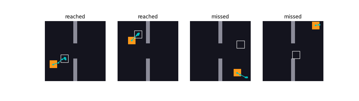
The plot shows four CEM episodes with the goal 8 steps ahead: two that reach the goal and two that miss it. The outline is the goal position of the agent.

paths, goals, miss = results[8, "CEM"]
episodes = [*np.flatnonzero(miss < 4)[:2], *np.flatnonzero(miss >= 4)[:2]]
fig, axes = plt.subplots(1, len(episodes), figsize=(3 * len(episodes), 3.4))
for ax, episode in zip(axes, episodes):
    path, goal = paths[episode], goals[episode]
    ax.imshow(world.render(path[0]).transpose(1, 2, 0), extent=(0, 64, 64, 0))
    ax.add_patch(Rectangle(goal, world.agent, world.agent, fill=False, color="w"))
    ax.plot(*(path + world.agent / 2).T, "c-o", markersize=3)
    ax.set_title("reached" if miss[episode] < 4 else "missed")
    ax.axis("off")
plt.show()

Limits of the planner

The planner works for near goals. For goals 16 steps ahead, the success rate is lower. The plot shows the reason. For pairs of random frames, it compares the distance between the two embeddings with the distance between the two agent positions.

positions = np.stack([world.random_position(rng) for _ in range(2000)])
embeddings = encode_positions(positions)
i, j = rng.integers(0, len(positions), size=(2, 20000))
pixel_distance = np.linalg.norm(positions[i] - positions[j], axis=1)
embedding_distance = (embeddings[i] - embeddings[j]).square().mean(dim=1).numpy()
bins = np.arange(0, 60, 4)
centers = [low + 2 for low in bins]
means = [
    embedding_distance[(pixel_distance >= low) & (pixel_distance < low + 4)].mean()
    for low in bins
]
plt.figure(figsize=(6, 4))
plt.plot(centers, means, marker="o")
plt.xlabel("distance between the agent positions (pixels)")
plt.ylabel("mean squared distance between the embeddings")
plt.show()

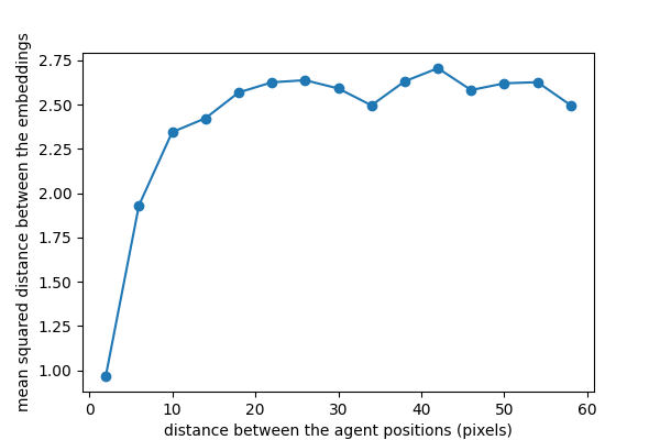
The embedding distance increases quickly for the first 10 pixels and then stays almost constant. For a goal that is 30 pixels away, most plans end in the flat part of the curve and have almost the same cost. CEM then finds the goal only if some of the sampled plans end near it. The LeWM paper reports a similar result on its Two-Room environment. The authors explain it with the low diversity and the low intrinsic dimension of the data. In this environment, the position of the agent is the only property that changes.

Other methods change the cost or the embeddings so that a planner can reach far goals:

• TEMPO trains a small model on frozen LeWM embeddings. In its space, the distance between two states is the number of steps between them. The planner uses this distance as the cost.

• PLDM trains with a loss term that keeps consecutive embeddings close, so that the embedding distance changes smoothly over time.

• Search on the Replay Buffer builds a graph of recorded states and plans a path of waypoints to the goal.

Next Steps

• LeWM describes the LeWM modules and the shapes of their inputs.

• LeJEPA uses the same SIGReg term for self-supervised learning on images.

• The official LeWM code trains LeWM on larger environments, for example Push-T and OGBench Cube.