Active Learning for Driveable Area Segmentation Using Cityscapes

Learn how to use active learning for driveable area segmentation using the BiSeNetV2 semantic segmentation model.

Driveable area detection is a common task for robotics applications. You want to know where your system can navigate to and where there might be obstacles. When deploying systems to the real world we often experience the issue that the real world performance heavily degrades once the model is used in an environment that differs from the training data. We call this issue "data drift" in the academic field around machine learning. The data seen in the production environment is drifting away from the training environment. An extreme example is a car that has only been trained in summer conditions that suddenly is deployed in winter conditions.

You will learn the following in this tutorial:

How to use a pre-trained BiSeNet open-source model for semantic segmentation and how to create predictions in the Lightly format.
Use metadata to balance the selected dataset across locations.
Access the results of a run directly using the API.

In this tutorial, we will make use of an image segmentation model for driveable area segmentation.

We will use the following model: https://github.com/CoinCheung/BiSeNet

Prerequisites

In order to upload predictions to a Lightly datasource, you will need the following things:

Have Lightly installed and setup.
Access to a cloud bucket to which you can upload your dataset. The following tutorial will use an AWS S3 bucket.
To use the BiSeNetV2 model, you can have a look at the official GitHub repository.
The cityscapes dataset. The dataset consists of 5 000 images for autonomous driving and is available on the official website. For the tutorial we need the train images in leftImg8bit_trainvaltest.zip and the vehicle metadata in vehicle_trainvaltest.zip.
We recommend using Python 3.7 or newer.

We assume the following file structure for the tutorial:

./
├── BiSeNet
│   ├── model_final_v2_city.pth
│   ├── prepare_predictions_and_metadata.py
│   ├── run_selection.py
│   └── ...
└── cityscapes
    ├── leftImg8bit
    │   └── train
    │       ├── aachen
    │       ├── ...
    │       └── zurich
    └── vehicle
        └── train
            ├── aachen
            ├── ...
            └── zurich

To download the BiSeNet code we use the following command:

git clone https://github.com/CoinCheung/BiSeNet
cd BiSeNet

All commands and scripts should be run from within the BiSeNet directory. For this tutorial, we want to start with an existing model checkpoint. We can either take the pretrained one from the repository or if you have your own checkpoint you can take that.

wget https://github.com/CoinCheung/BiSeNet/releases/download/0.0.0/model_final_v2_city.pth

Run a prediction using the BiSeNet Segmentation Model

Before jumping into active learning let's try to get the model running on a random image from cityscapes. We prepared the most essential code in the following snippet. This will do the following:

load the model from the checkpoint
load an image from cityscapes
preprocess the image (normalize + resize)
run inference
drop all classes we don't care about (we just want to predict driveable area here)
store the prediction as an image

import json
import math
from pathlib import Path

import cv2
import numpy as np
import torch
import torch.nn as nn
import torch.nn.functional as F
import tqdm
from PIL import Image

import lib.data.transform_cv2 as T
from lib.models import model_factory

# set dataset paths
cityscapes_dir = Path("../cityscapes")
image_dir = cityscapes_dir / "leftImg8bit"
vehicle_dir = cityscapes_dir / "vehicle"

## define bisenetv2 model
# config taken from BiSeNet/configs/bisenetv2_city.py
net = model_factory["bisenetv2"](19, aux_mode="eval")
net.load_state_dict(
    torch.load("model_final_v2_city.pth", map_location="cpu"), strict=False
)
net.eval()
net.cuda()

# example image name and color palette (road, background)
example_image_fname = image_dir / "train/aachen/aachen_000000_000019_leftImg8bit.png"
palette = np.array([[128, 64, 128], [0, 0, 0]])


def run_inference(img_fname: str, model: nn.Module) -> np.ndarray:
    """Loads image from filename and runs inference using model."""
    # to normalize the data
    to_tensor = T.ToTensor(
        mean=(0.3257, 0.3690, 0.3223),  # cityscapes, rgb
        std=(0.2112, 0.2148, 0.2115),
    )
    im = cv2.imread(img_fname)[:, :, ::-1]
    im = to_tensor(dict(im=im, lb=None))["im"].unsqueeze(0).cuda()

    # shape divisor
    org_size = im.size()[2:]
    new_size = [math.ceil(el / 32) * 32 for el in im.size()[2:]]

    # inference
    im = F.interpolate(im, size=new_size, align_corners=False, mode="bilinear")

    with torch.no_grad():
        out = model(im)[0]

    out = torch.nn.functional.softmax(out, 1)

    # Simplify the output to only two classes: road and not road.
    # We do this by taking the max over all classes except road.
    # The road class is the first class (trainId = index = 0).
    # You can find all labels here:
    # https://github.com/CoinCheung/BiSeNet/blob/master/lib/data/cityscapes_cv2.py
    out_class_road = out[:, 0, :, :]
    out_other_classes_max = torch.max(out[:, 1:, :, :], dim=1)[0]
    out_merged = torch.stack([out_class_road, out_other_classes_max], dim=1)

    out_scaled = F.interpolate(out_merged, size=org_size, align_corners=False, mode="bilinear")

    return out_scaled


out = run_inference(str(example_image_fname), net)

# visualize
out_scaled = out.argmax(dim=1)
out_scaled = out_scaled.squeeze().detach().cpu().numpy()
pred = palette[out_scaled]
cv2.imwrite("./example_prediction.jpg", pred)

After running the code we should see a new image with the name example_prediction.jpg containing our prediction. The original image we used for the prediction is ../data/train/aachen/aachen_000000_000019_leftImg8bit.png. You can see both, the input image and the prediction in the image below.

800 — The segmentation output of our model next to the input image. As you can see our model is pretty accurate in detecting roads.

Get Predictions for Cityscapes using BiSeNet

Now we want to use the model output for active learning with Lightly. Since segmentation model outputs can be very large in dimensions we want to compress this information a bit.

📘
Size of Semantic Segmentation Predictions
The model used in this tutorial would without any tricks create a 1024x2048x19 tensor with floating point values. Using 4 Bytes per float (32 bit precision) we end up with 152MBytes per prediction.
It's not feasible to work with such large files. If we would just use the argmax instead we would get a 1024x2048 tensor we can nicely compress using formats such as png as we would no longer have arbitrary float values but only integers.
In order to still be able to tell about the probability of the prediction we use a combination of both. We use the so-called RLE (Run Length Encoding) format that allows us to store data in a more efficient way. Additionally, we store the prediction probability as a separate value for each RLE segment.

We provide the following two helper functions to turn a raw prediction into the correct format Lightly can work with.

def binary_to_rle_torch(binary_mask: torch.Tensor) -> torch.Tensor:
    """Converts a binary segmentation mask of shape H x W to RLE."""
    # Flatten mask and add -1 at beginning and end of array
    tensor_minus_1 = torch.IntTensor([-1]).to(binary_mask.device)
    tensor_zero = torch.IntTensor([0]).to(binary_mask.device)

    flat = torch.cat((tensor_minus_1, torch.ravel(binary_mask), tensor_minus_1))
    # Find indices where a change to 0 or 1 happens
    borders = torch.nonzero(torch.diff(flat)).squeeze(1)
    # Find counts of subsequent 0s and 1s
    rle = torch.diff(borders)
    if flat[1]:
        # The first value in the encoding must always be the count
        # of initial 0s. If the mask starts with a 1 we must set
        # this count to 0.
        rle = torch.cat((tensor_zero, rle))
    return rle

def convert_to_lightly_prediction_torch(filename: str, seg_map: torch.Tensor):
    """Converts a segmentation map of shape H x W x C to Lightly format."""
    seg_map_argmax = torch.argmax(seg_map, dim=2)

    prediction = {"file_name": filename, "predictions": []}
    for category_id in torch.unique(seg_map_argmax):
        rle = binary_to_rle_torch(seg_map_argmax == category_id)
        logits = torch.mean(seg_map[seg_map_argmax == category_id], dim=0)
        assert torch.argmax(logits) == category_id
        probabilities = torch.exp(logits) / torch.sum(torch.exp(logits))
        assert abs(torch.sum(probabilities) - 1.0) < 1e-6

        prediction["predictions"].append(
            {
                "category_id": int(category_id.item()),
                "segmentation": [int(r.item()) for r in rle],
                "score": float(probabilities[category_id].item()),
                "probabilities": [float(p.item()) for p in probabilities],
            }
        )

    return prediction

Finally, we can loop through the dataset and use the helper functions from above to get predictions in the right format. This process should take 10-15 minutes on a GPU.

# create predictions folder and add tasks.json and schema.json
predictions_root_path = Path("predictions")
task_name = "segmentation_cityscapes"
predictions_path = predictions_root_path / task_name

# create tasks.json
tasks_json_path = predictions_root_path / "tasks.json"
tasks_json_path.parent.mkdir(parents=True, exist_ok=True)

with open(tasks_json_path, "w") as f:
    json.dump([task_name], f)


# create schema.json
schema = {
    "task_type": "semantic-segmentation",
    "categories": [{"id": 0, "name": "road"}, {"id": 1, "name": "not road"}],
}

schema_path = predictions_path / "schema.json"
schema_path.parent.mkdir(parents=True, exist_ok=True)

with open(schema_path, "w") as f:
    json.dump(schema, f, indent=4)

fnames = list(image_dir.glob("train/**/*.png"))

for fname in tqdm.tqdm(fnames):
    out = run_inference(str(fname), net)
    # change shape from [1, 19, 1024, 2048] to [1024, 2048, 19]
    seg_map = out.squeeze(0).permute(1, 2, 0)
    img_relative_fname = fname.relative_to(image_dir)
    pred = convert_to_lightly_prediction_torch(str(img_relative_fname), seg_map)

    out_fname = predictions_path / img_relative_fname.with_suffix(".json")
    out_fname.parent.mkdir(parents=True, exist_ok=True)
    with open(out_fname, "w") as f:
        json.dump(pred, f)

Get Metadata from Cityscapes in Lightly Format

For Cityscapes, the authors also provide metadata. In fact, for autonomous robots, we very often have access to sensor values ranging from motion sensors, GPS, camera identifiers, etc.

In this example, we want to use all the provided metadata and also use the folder name (which is the name of the city) as additional metadata and use it with Lightly.

# create metadata schema.json
schema = [
    {
        "name": "City",
        "path": "city",
        "defaultValue": "undefined",
        "valueDataType": "CATEGORICAL_STRING",
    },
    {
        "name": "GPS Heading",
        "path": "vehicle.gpsHeading",
        "defaultValue": -1,
        "valueDataType": "NUMERIC_INT",
    },
    {
        "name": "Latitude",
        "path": "vehicle.gpsLatitude",
        "defaultValue": -1,
        "valueDataType": "NUMERIC_FLOAT",
    },
    {
        "name": "Longitude",
        "path": "vehicle.gpsLongitude",
        "defaultValue": -1,
        "valueDataType": "NUMERIC_FLOAT",
    },
    {
        "name": "Outside Temperature",
        "path": "vehicle.outsideTemperature",
        "defaultValue": -1,
        "valueDataType": "NUMERIC_FLOAT",
    },
    {
        "name": "Speed",
        "path": "vehicle.speed",
        "defaultValue": -1,
        "valueDataType": "NUMERIC_FLOAT",
    },
    {
        "name": "Yaw Rate",
        "path": "vehicle.yawRate",
        "defaultValue": -1,
        "valueDataType": "NUMERIC_FLOAT",
    },
]

schema_path = Path("metadata/schema.json")
schema_path.parent.mkdir(parents=True, exist_ok=True)

with open(schema_path, "w") as f:
    json.dump(schema, f, indent=4)

fnames = list(image_dir.glob("train/**/*.png"))


def get_city_from_fname(fname: Path) -> str:
    return str(fname.parent.name)


for fname in tqdm.tqdm(fnames):
    vehicle_metadata_fname = vehicle_dir / fname.relative_to(image_dir)
    vehicle_metadata_fname = str(vehicle_metadata_fname.with_suffix(".json")).replace(
        "leftImg8bit", "vehicle"
    )

    with open(vehicle_metadata_fname, "r") as f:
        vehicle_metadata = json.load(f)

    metadata = {
        "file_name": str(fname.relative_to(image_dir)),
        "type": "image",
        "metadata": {"city": get_city_from_fname(fname), "vehicle": vehicle_metadata},
    }

    lightly_metadata_fname = "metadata" / fname.relative_to(image_dir).with_suffix(
        ".json"
    )
    lightly_metadata_fname.parent.mkdir(parents=True, exist_ok=True)

    with open(lightly_metadata_fname, "w") as f:
        json.dump(metadata, f, indent=4)

A metadata JSON file could look like the following:

{
    "file_name": "train/aachen/aachen_000000_000019_leftImg8bit.png",
    "type": "image",
    "metadata": {
        "city": "aachen",
        "vehicle": {
            "gpsHeading": 281,
            "gpsLatitude": 50.780881831805594,
            "gpsLongitude": 6.108147476339736,
            "outsideTemperature": 19.5,
            "speed": 10.814562500000001,
            "yawRate": 0.17090297010894437
        }
    }
}

Optional: Upload to AWS Bucket

Now, we can upload the predictions and images to the cloud to process them using Lightly. We use AWS in this example but other cloud providers such as GCP or Azure are also fully supported.

First, we upload the dataset:

aws s3 cp ../cityscapes/leftImg8bit/train/ s3://yourInputBucket/cityscapes_input/train --recursive

Now, we can upload the predictions:

aws s3 cp predictions/ s3://yourLightlyBucket/cityscapes_lightly/.lightly/predictions --recursive

Finally, we can upload the metadata using:

aws s3 cp metadata/ s3://yourLightlyBucket/cityscapes_lightly/.lightly/metadata --recursive

At this point, your final bucket structure should look similar to the one below. Note that the folder hierarchy within the metadata or predictions folders matches the structure of the input bucket.

s3://yourInputBucket/cityscapes_input/
└── train/
    ├── aachen/
    │   ├── aachen_000000_000019_leftImg8bit.png
    │   ├── ...
    │   └── aachen_000173_000019_leftImg8bit.png
    ├── ...
    └── zurich/
        └── ...

s3://yourLightlyBucket/cityscapes_lightly/
└── .lightly/
    ├── metadata/
    │   └── train/
    │       └── aachen/
    │           ├── aachen_000000_000019_leftImg8bit.json
    │           ├── ...
    │           └── aachen_000173_000019_leftImg8bit.json
    │       ├── ...
    │       └── zurich/
    │           └── ...
    └── predictions/
        ├── segmentation_cityscapes/
        │   ├── schema.json
        │   └── train/
        │       ├── aachen/
        │       │   ├── aachen_000000_000019_leftImg8bit.json
        │       │   ├── ...
        │       │   └── aachen_000173_000019_leftImg8bit.json
        │       ├── ...
        │       └── zurich/
        │           └── ...
        └── tasks.json

Run Selection

Now, we have the data prepared and ready to be processed. As a next step we can start the Lightly Worker to get ready for processing the new jobs we will submit using another Python script shortly. Note, that you can also start the Lightly Worker later but nothing can be processed until a worker is running.

docker run --shm-size="1024m" --gpus all --rm -it \
	  -e LIGHTLY_TOKEN={MY_LIGHTLY_TOKEN} \
	  -e LIGHTLY_WORKER_ID={MY_WORKER_ID} \
	  lightly/worker:latest \

As a final step, we can now submit the job for processing. We recommend putting the dataset creation, datasource configuration, and job submission into a single script. Optionally, you can also use the compute_worker_run_info_generator to monitor the job (the script would then run until the job is completed).

The provided configuration does the following:

We fine-tune a self-supervised learning model for 25 epochs on the dataset to get good embeddings
We select data based on the following three criteria
- We want diverse images by using embeddings.
- We want to select images where the prediction entropy is high (Active Learning).
- We want to balance the selected images equally among the cities.

Please don't forget also here to update the individual placeholders for the authentication and datasources!

from pathlib import Path

from lightly.api import ApiWorkflowClient
from lightly.openapi_generated.swagger_client import DatasetType
from lightly.openapi_generated.swagger_client import DatasourcePurpose


# Create the Lightly client to connect to the API.
client = ApiWorkflowClient(token="MY_LIGHTLY_TOKEN")

# Create a new dataset on the Lightly Platform.
client.create_dataset(
    dataset_name="cityscapes_tutorial", dataset_type=DatasetType.IMAGES
)
dataset_id = client.dataset_id

# Configure the Input datasource.
client.set_s3_delegated_access_config(
    resource_path="s3://yourInputBucket/cityscapes_input/",
    region="us-west-2",
    role_arn="S3-ROLE-ARN",
    external_id="S3-EXTERNAL-ID",
    purpose=DatasourcePurpose.INPUT,
)
# Configure the Lightly datasource.
client.set_s3_delegated_access_config(
    resource_path="s3://yourLightlyBucket/cityscapes_lightly/",
    region="us-west-2",
    role_arn="S3-ROLE-ARN",
    external_id="S3-EXTERNAL-ID",
    purpose=DatasourcePurpose.LIGHTLY,
)

# set dataset paths
cityscapes_dir = Path("../cityscapes")
image_dir = cityscapes_dir / "leftImg8bit"

# we get a list of cities using the folders in train
cities = list(image_dir.glob("train/*"))

scheduled_run_id = client.schedule_compute_worker_run(
    worker_config={
        "enable_training": True,
    },
    selection_config={
        "n_samples": 2000,
        "strategies": [
            {
                # strategy to find diverse images
                "input": {
                    "type": "EMBEDDINGS",
                },
                "strategy": {
                    "type": "DIVERSITY",
                },
            },
            {
                # strategy to use prediction score (Active Learning)
                "input": {
                    "type": "SCORES",
                    "task": "segmentation_cityscapes",
                    "score": "uncertainty_entropy",
                },
                "strategy": {"type": "WEIGHTS"},
            },
            {
              	# strategy to balance across the cities
                "input": {"type": "METADATA", "key": "city"},
                "strategy": {
                    "type": "BALANCE",
                    "target": {str(city.name): 1 / len(cities) for city in cities},
                },
            },
        ],
    },
    lightly_config={
        "trainer": {
            "max_epochs": 25,
        },
        "loader": {"batch_size": 128},
    },
)

# You can use this code to track and print the state of the Lightly Worker.
# The loop will end once the run has finished, was canceled, or failed.
for run_info in client.compute_worker_run_info_generator(
    scheduled_run_id=scheduled_run_id
):
    print(
        f"Lightly Worker run is now in state='{run_info.state}' with message='{run_info.message}'"
    )

if run_info.ended_successfully():
    print("SUCCESS")
else:
    print("FAILURE")

Analyze the Results

Whenever you process a dataset with Lightly, you will have access to the following results:

A completed Lightly Worker run with artifacts such as model checkpoints and logs.
A PDF report that summarizes what data has been selected and why.
Furthermore, our dataset in the Lightly Platform contains now the selected images.

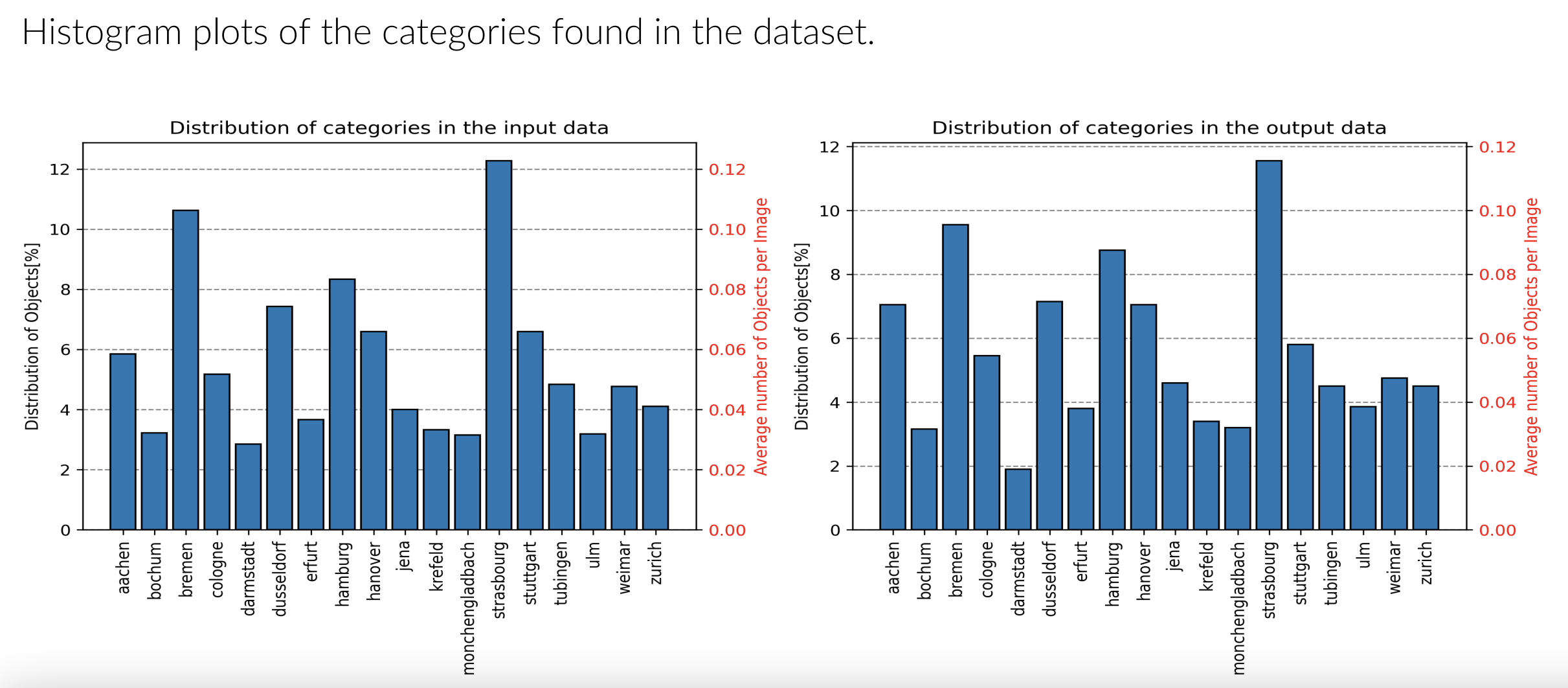
In the PDF report we can find information about the distribution change between the input data and the selected data. As you can see the distribution only slightly changed. Data from the city of Strasbourg was overly represented in the input data and by using balancing the selected portion contains now less than 12% (vs more than 12% before) of this location. However, for the city of Darmstadt the ratio decreased from over 2% to below 2%.

2422 — Metadata distribution in the input and selected data.

We can now use the Lightly Platform to visually explore the difference between the two cities (Strasbourg and Darmstadt) in the embedding space.

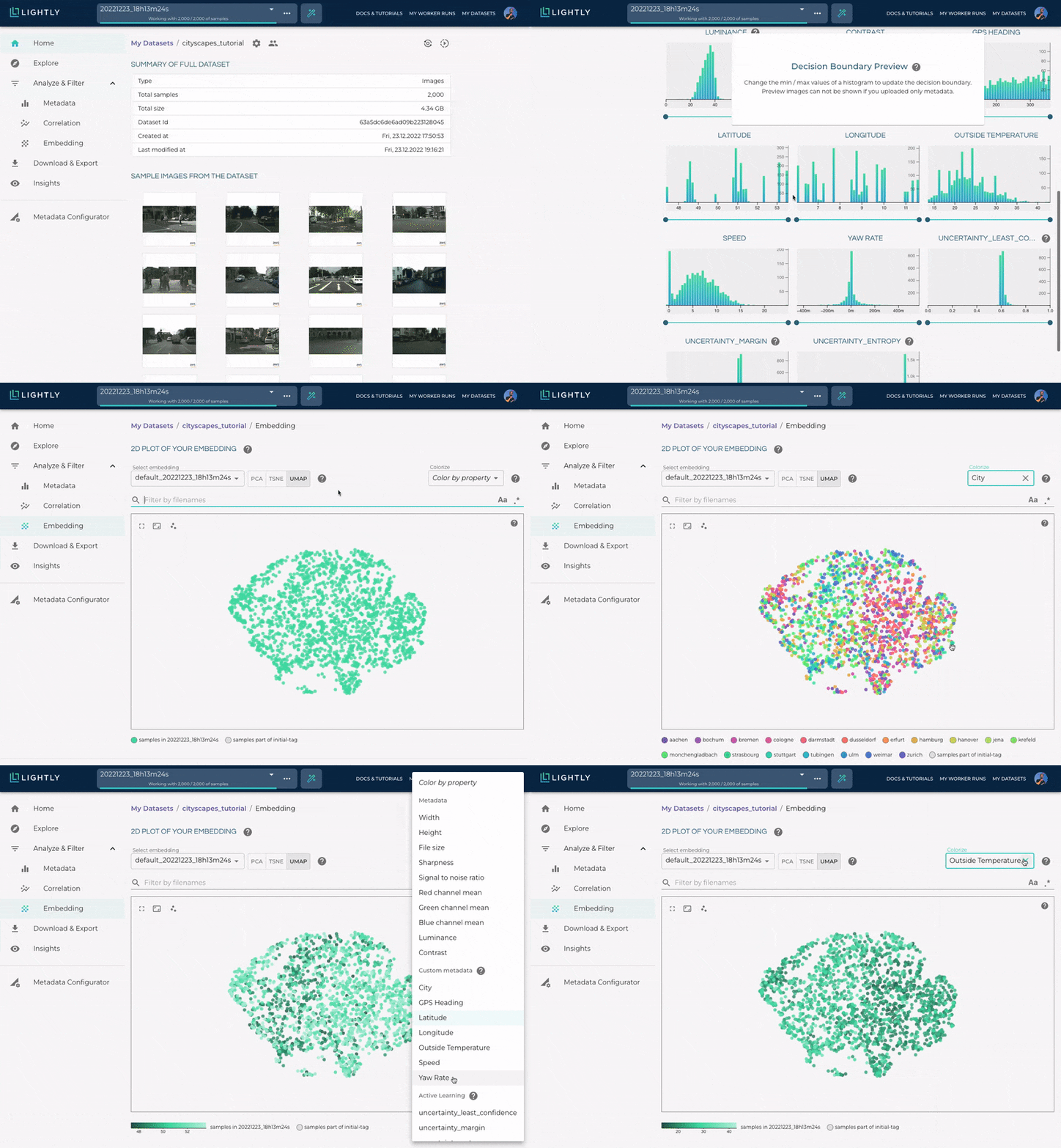
The Lightly Platform can help us to further analyze the selected data. You can explore the embeddings and metadata interactively.

800 — The Lightly Platform can be very helpful to visualize the selected data. Find interesting edge cases and get insights about the data distribution.

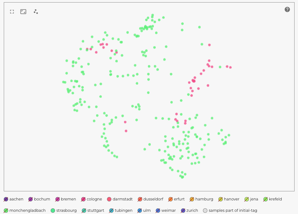
In the embedding view we can select "color by property" on the top right and click on city. Then we can click on the different cities in the legend (below the embedding plot) to hide them. Finally, we can look at the embeddings of Strasbourg and Darmstadt. We notice, that the data from Strasbourg (green color) is more diverse and covering more of the embedding space than Darmstadt (pink).

947 — Use the embedding view to compare the distribution of the two cities Strasbourg and Darmstadt.

Download the Run Artifacts of our Cityscapes Tutorial

We can access the run artifacts as well as the list of the 2'000 selected filenames using the api client. Since every dataset can have several runs we only load the latest one here.

To download the artifacts we use the lightly api client API.

from lightly.api import ApiWorkflowClient
import json

# Create the Lightly client to connect to the API. 
# You can also combine this with the script above and reuse the client.
client = ApiWorkflowClient(token="MY_LIGHTLY_TOKEN", dataset_id="MY_DATASET_ID")

# get all runs for a given dataset sorted from old to new
runs = client.get_compute_worker_runs(dataset_id=client.dataset_id)
run = runs[-1] # get the latest run

# download all artifacts to "my_run/artifacts"
client.download_compute_worker_run_artifacts(run=run, output_dir="my_run/artifacts")

# instead of downloading all artifacts we can also only access the files we want
# e.g. to just download the report pdf
# client.download_compute_worker_run_report_pdf(run=run, output_path="report.pdf")
# for more info: https://docs.lightly.ai/self-supervised-learning/lightly.api.html

# finally, we also want to get the filenames with signed read URLs
filenames_and_read_urls = client.export_filenames_and_read_urls_by_tag_name(
    tag_name="initial-tag"  # name of the tag in the dataset
)
with open("filenames-and-readurls-of-initial-tag.json", "w") as f:
    json.dump(filenames_and_read_urls, f)