Active Learning Using YOLOv7 and Comma10k
Use this complete guide for active learning using LightlyOne and YOLOv7 for your next computer vision object detection project.
When developing new computer vision solutions, we often rely on transfer learning (we use a pre-trained model and transfer it to a new task). For transfer learning, we require significantly fewer labeled examples. It's therefore a great way to kick off new projects. However, we still need to fine-tune our model using supervised learning.
Why should I use Active Learning in Computer Vision?
When working with images, data labeling can be very time-consuming and expensive. But we need labeled data for fine-tuning our model. In order to reduce the amount of data required for fine-tuning, we can use active learning using the model predictions to find the most relevant data. With Lightly, we can take this even one step further and combine model predictions with embeddings to find "difficult" images with diverse objects.
In this example, we show how to use LightlyOne to select the most relevant images to be used for labeling and transfer learning of your model. We do this by uploading predictions to LightlyOne and using them to do Active Learning.
You will learn the following in this tutorial:
- How to use pre-trained YOLOv7 open-source model to create predictions in the Lightly format.
- Learn how to use the selection config of the LightlyOne Solution to find the best images for labeling.
- Learn how to interpret the results of a run.
Prerequisites
In order to upload predictions to a Lightly datasource, you will need the following things:
- Have LightlyOne installed and setup.
- Access to a cloud bucket to which you can upload your dataset. The following tutorial will use an AWS S3 bucket.
- To use the YOLOv7 model, you can have a look at the official GitHub repository.
- The comma10k dataset. The dataset consists of
10 000images for autonomous driving and is available on GitHub. You can download the dataset using git (~24GB of size). - We recommend using
Python 3.7or newer.
Downloading the Comma10k Dataset
To download the Comma10k dataset, we can run the following command in our terminal:
git clone https://github.com/commaai/comma10kTo download the YOLOv7 code we use the following command:
git clone https://github.com/WongKinYiu/yolov7In case you don't have a Python environment with PyTorch and some other dependencies installed, we recommend running pip install -r yolov7/requirements.txt and pip install lightly to install all the required dependencies.
We also need a model checkpoint. We can get the one from the repository using the following command:
cd yolov7 && wget https://github.com/WongKinYiu/yolov7/releases/download/v0.1/yolov7.ptFrom this point on we assume that you have the following folder structure:
yolov7/
└── ...
comma10k/
└── ...
Now we have a model and the dataset. Let's use the YOLOv7 model on a single image to make a prediction and see how things work and look.
We already prepared a minimal script to run the model. You can save this file within the YOLOv7 directory and then run it using Python with python single_prediction.py.
import torch
import torchvision
import cv2

from models.experimental import attempt_load
from utils.torch_utils import select_device
from utils.general import check_img_size, non_max_suppression
from utils.datasets import LoadImages

device = select_device()

model = attempt_load("./yolov7.pt", map_location=device)  # load FP32 model
stride = int(model.stride.max())  # model stride
imgsz = check_img_size(640, s=stride)  # check img_size

dataset = LoadImages(
    "../comma10k/imgs/7000_033036500e8ede52_2018-09-14--14-05-49_49_718.png",
    img_size=640,
    stride=32,
)

for path, img, im0s, vid_cap in dataset:
    img = torch.from_numpy(img).to(device).float().unsqueeze(0)
    img /= 255.0
    with torch.no_grad():
        output = model(img)[0]

    predictions = non_max_suppression(output, conf_thres=0.25, iou_thres=0.45)[0]

    # each prediction has format [x0, y0, x1, y1, conf, class_index]
    # the bounding box coordinates are in pixels and [0,0] is top left
    print(predictions)

bboxes = predictions[:, :4]
labels = [str(int(label)) for label in predictions[:, 5].data]

img_pred = torchvision.utils.draw_bounding_boxes(
    (img[0] * 255).to(torch.uint8), bboxes, labels
).numpy()

# we need to convert from CxHxW to HxWxC
img_pred = img_pred.transpose((1, 2, 0))

cv2.imwrite("img_with_predictions.jpg", img_pred)
If you run the script above within the yolov7 folder, you should get a similar result to the one below. There are a few log statements from building the YOLOv7 model, followed by our print statement about the model predictions.
Fusing layers...
RepConv.fuse_repvgg_block
RepConv.fuse_repvgg_block
RepConv.fuse_repvgg_block
tensor([[3.43357e+02, 2.29525e+02, 3.65856e+02, 2.47247e+02, 8.70795e-01, 2.00000e+00],
        [3.72252e+02, 2.15537e+02, 4.51338e+02, 2.68655e+02, 7.97245e-01, 7.00000e+00],
        [7.56669e+01, 2.29587e+02, 1.10844e+02, 2.41963e+02, 7.71481e-01, 2.00000e+00],
        [1.91022e+02, 2.18533e+02, 2.52842e+02, 2.65889e+02, 6.88630e-01, 2.00000e+00],
        [2.90663e+02, 2.26180e+02, 3.18073e+02, 2.53414e+02, 6.59410e-01, 2.00000e+00],
        [7.40601e-01, 2.29518e+02, 4.83450e+01, 2.44514e+02, 6.22376e-01, 2.00000e+00],
        [3.19597e+02, 2.13846e+02, 3.39611e+02, 2.38194e+02, 5.75851e-01, 7.00000e+00],
        [3.31235e+02, 2.19448e+02, 3.52366e+02, 2.41629e+02, 5.59704e-01, 7.00000e+00],
        [1.77030e+02, 2.28873e+02, 1.94312e+02, 2.42095e+02, 5.11743e-01, 2.00000e+00],
        [1.18014e+02, 2.23159e+02, 1.62899e+02, 2.40230e+02, 4.98371e-01, 2.00000e+00],
        [1.90748e+02, 2.18261e+02, 2.52851e+02, 2.65495e+02, 3.76240e-01, 7.00000e+00],
        [1.18875e+02, 2.23032e+02, 1.67154e+02, 2.40521e+02, 3.41600e-01, 7.00000e+00],
        [2.91023e+02, 2.22591e+02, 3.18455e+02, 2.53489e+02, 3.20579e-01, 7.00000e+00],
        [3.73559e+02, 2.15982e+02, 4.50630e+02, 2.68176e+02, 3.12213e-01, 2.00000e+00],
        [1.11107e+02, 2.30915e+02, 1.43412e+02, 2.40902e+02, 2.55858e-01, 2.00000e+00]], device='cuda:0')
YOLOv7 Prediction OutputPlease note that the output format of YOLOv7 after non-maximum suppression (NMS) has the following structure:
[x_min, y_min, x_max, y_max, conf, class_index]The bounding box coordinates are pixel coordinates, and they are scaled based on the input image size. Since we resized the image before feeding it through the model, we will need to rescale the bounding box coordinates to get the correct values. We will do this later using the
scale_coordsmethod of theyolov7codebase we're using.
Additionally, we use the draw_bounding_boxes method of torchvision to draw bounding boxes on the image and save the result as img_with_predictions.jpg. As you see, our model is able to detect many objects correctly in the scene
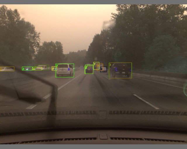
Example prediction from our YOLOv7 model on the Comma10k dataset. The numbers next to the bounding boxes indicate the label index of the class. 2 is car and 7 is truck.
Prepare the YOLOv7 Predictions
After testing that our model works and does what we want, we can start creating predictions for the whole dataset, so we can use them for active learning with Lightly.
Computing the predictions consists of the following two steps:
- Run the model over the data to get predictions.
- Add tasks and schema in the Lightly format.
Get Predictions for All Images
We can reuse the code from our example of running a first prediction to quickly loop over the whole dataset and get predictions. We will need to bring the predictions into the prediction format as outlined at Prediction Format:
{
    "predictions": [ // classes: [person, car]
        {
            "category_id": 0,           // category in [0, num categories - 1]
            "bbox": [140, 100, 80, 90], // x, y, w, h coordinates in pixels
                                        // x, y >= 0 and w, h >= 1
            "score": 0.8,               // prediction score in [0, 1]
            "probabilities": [0.2, 0.8] // optional, values in [0, 1], sum up to 1.0
        },
        {
            "category_id": 1,
            "bbox": [...],
            "score": 0.9,
            "probabilities": [0.9, 0.1] // optional, sum up to 1.0
        }
    ]
}
Let's modify the code to get the predictions and convert them to the right format. To get the most out of Lightlys' active learning capabilities, we can increase the number of false positive and false negative predictions. We can do this by simply reducing the conf_thres and increasing the iou_thres during non-maximum suppression.
- A lower
conf_threskeeps more predictions based on their objectness probability. - A higher
iou_thrsresults in fewer overlapping bounding boxes.
You can also keep the YOLOv7 default values.

By changing the iou_thres for our YOLOv7 prediction we decide on whether we want to keep overlapping bounding boxes or not. We remove two bounding boxes if their IoU is greater than iou_thres. We show here three examples for a threshold of 0.05, 0.45 and 0.95.
Furthermore, we only care about a handful of classes of the MSCOCO pretrained model.
Classes we want to keep: ['person', 'bicycle', 'car', 'motorcycle', 'bus', 'train', 'truck']. We can find the index of these classes from the data/coco.yaml file.
In the following script, we do three things:
- Create a
tasks.jsonfile with the object detection task. - Create a
schema.jsonfor the object detection prediction schema. - Run the YOLOv7 model on the whole dataset to get predictions and dump them in the right format.
from pathlib import Path
import json

import torch
import torchvision
import cv2
from tqdm import tqdm

from models.experimental import attempt_load
from utils.torch_utils import select_device
from utils.general import check_img_size, non_max_suppression, scale_coords
from utils.datasets import LoadImages

predictions_rooth_path = Path("predictions")
task_name = "object_detection_comma10k"
predictions_path = Path(predictions_rooth_path / task_name)

important_classes = {
    "person": 0,
    "bicycle": 1,
    "car": 2,
    "motorcycle": 3,
    "bus": 5,
    "train": 6,
    "truck": 7,
}

classes = list(important_classes.values())

# create tasks.json
tasks_json_path = predictions_rooth_path / "tasks.json"
tasks_json_path.parent.mkdir(parents=True, exist_ok=True)

with open(tasks_json_path, "w") as f:
    json.dump([task_name], f)


# create schema.json
schema = {"task_type": "object-detection", "categories": []}
for key, val in important_classes.items():
    cat = {"id": val, "name": key}
    schema["categories"].append(cat)

schema_path = predictions_path / "schema.json"
schema_path.parent.mkdir(parents=True, exist_ok=True)

with open(schema_path, "w") as f:
    json.dump(schema, f, indent=4)


device = select_device()

model = attempt_load("./yolov7.pt", map_location=device)  # load FP32 model
stride = int(model.stride.max())  # model stride
imgsz = check_img_size(640, s=stride)  # check img_size

dataset = LoadImages(
    "../comma10k/imgs/",  # here we use the folder instead of a single image
    img_size=640,
    stride=32,
)

for path, img, im0s, vid_cap in tqdm(dataset):
    img = torch.from_numpy(img).to(device).float().unsqueeze(0)
    img /= 255.0
    with torch.no_grad():
        prediction = model(img)[0]

    # apply NMS and only keep classes we care about (see data/coco.yaml)
    predictions = non_max_suppression(
        prediction, conf_thres=0.25, iou_thres=0.45, classes=classes
    )[0]

    fname = Path(path).name

    lightly_prediction = {
        "predictions": [],
    }

    # we need to rescale the bounding boxes as inference was done
    # on resized and padded images
    predictions[:, :4] = scale_coords(
        img.shape[2:], predictions[:, :4], im0s.shape
    ).round()

    for prediction in predictions:
        x0, y0, x1, y1, conf, class_id = prediction.cpu().numpy()

        # note that we need to convert form x0, y0, x1, y1 to x, y, w, h format
        pred = {
            "category_id": int(class_id),
            "bbox": [int(x0), int(y0), int(x1 - x0), int(y1 - y0)],
            "score": float(conf),
        }
        lightly_prediction["predictions"].append(pred)

        # create the prediction file for the image
        path_to_prediction = predictions_path / Path(fname).with_suffix(".json")

        path_to_prediction.parents[0].mkdir(parents=True, exist_ok=True)
        with open(path_to_prediction, "w") as f:
            json.dump(lightly_prediction, f, indent=4)
The resulting folder structure should look like this:
predictions/
├── tasks.json
└── object_detection_comma10k/
    ├── schema.json
    ├── 0000_0085e9e41513078a_2018-08-19--13-26-08_11_864.json
    ├── ...
    └──  0999_e8e95b54ed6116a6_2018-10-22--11-26-21_3_339.json
Prepare Dataset and Predictions
To do Active Learning, use Object Diversity. The dataset and predictions must be accessible to Lightly. You need to upload the data to a cloud provider of your choice. For this tutorial, you can use AWS S3. LightlyOne also supports Google Cloud Storage or Azure.
Set Up Your S3 Bucket
If you haven't done it already, follow the instructions here to set up an input and Lightly datasource on S3.
Optional: Upload Data to Bucket using AWS CLI
Install AWS CLI
We suggest you use AWS CLI to upload your dataset and predictions because it is faster for uploading large numbers of images. You can find the tutorial on installing the CLI on your system here. Test if AWS CLI was installed successfully with:
which aws
aws --version
After successful installation, you also need to configure the AWS CLI and enter your IAM credentials:
aws configureUpload Dataset and Predictions
Now you can copy the content of your dataset to your cloud bucket with the aws s3 cp command. We will copy both the content in the comma10k and the lightly_comma10k folders.
# verified and works
aws s3 cp imgs s3://bucket/input/comma10k/ --recursive
aws s3 cp predictions/ s3://bucket/lightly/comma10k/.lightly/predictions --recursive
Replace the PlaceholderMake sure you don't forget to replace the placeholders
s3://bucket/inputands3://bucket/lightlywith the name of your AWS S3 bucket paths.
Example of Folder Structure in AWS
Here is the final structure of your files on AWS S3:
s3://bucket/input/comma10k/
├── 0000_0085e9e41513078a_2018-08-19--13-26-08_11_864.png
├── ...
└── 0999_e8e95b54ed6116a6_2018-10-22--11-26-21_3_339.png

s3://bucket/lightly/comma10k/
└── .lightly/predictions/
    ├── tasks.json
    └── object_detection_comma10k/
          ├── schema.json
          ├── 0000_0085e9e41513078a_2018-08-19--13-26-08_11_864.json
          ├── ...
          └── 0999_e8e95b54ed6116a6_2018-10-22--11-26-21_3_339.json
Now you have your dataset and predictions ready to be used by the LightlyOne Worker!
Select Data using Predictions
After setting up the data, we can finally create the run to process it and select the desired subset. Using LightlyOne to process datasets consists of three parts:
- Start the LightlyOne Worker.
- Create a new dataset and configure a datasource.
- Schedule a run.
Start the LightlyOne Worker
Now, we can start our LightlyOne Worker. The worker will wait for new jobs to be processed. The cool thing about this setup is that we can start the LightlyOne Worker on any machine. You could, for example, use your cloud instance with a GPU or a local server to run the LightlyOne Worker while using your notebook to schedule the run :)
docker run --shm-size="1024m" --gpus all --rm -it \
	-e LIGHTLY_TOKEN="MY_LIGHTLY_TOKEN" \
	lightly/worker:latest
Use your Lightly Token and Worker IdDon't forget to replace the
{MY_LIGHTLY_TOKEN}placeholder with your own token. In case you forgot your token, you can find your token in the preferences menu of the LightlyOne Platform.
Create the Dataset and Datasource
We suggest putting the remaining four code snippets into a single Python script.
In the first part, we import the dependencies, and we create a new dataset.
from lightly.api import ApiWorkflowClient
from lightly.openapi_generated.swagger_client import DatasetType
from lightly.openapi_generated.swagger_client import DatasourcePurpose

# Create the Lightly client to connect to the API.
client = ApiWorkflowClient(token="MY_LIGHTLY_TOKEN")

# Create a new dataset on the LightlyOne Platform.
client.create_dataset(dataset_name="comma10k", dataset_type=DatasetType.IMAGES)
dataset_id = client.dataset_id# Configure the Input datasource.
client.set_s3_delegated_access_config(
resource_path="s3://bucket/input/comma10k/",
region="eu-central-1",
role_arn="S3-ROLE-ARN",
external_id="S3-EXTERNAL-ID",
purpose=DatasourcePurpose.INPUT,
)
# Configure the Lightly datasource.
client.set_s3_delegated_access_config(
resource_path="s3://bucket/lightly/comma10k/",
region="eu-central-1",
role_arn="S3-ROLE-ARN",
external_id="S3-EXTERNAL-ID",
purpose=DatasourcePurpose.LIGHTLY,
)Schedule a Run
Finally, we can schedule a LightlyOne Worker run to select a subset of the data based on our criteria. Since we have access to the predictions, we will use them threefold.
- We use predictions to balance the ratio of the classes.
- We use predictions to create embeddings of the objects within the bounding boxes to find diverse objects.
- We use predictions to focus on objects where the probability of the prediction is low (Active Learning).
- We train an embedding model for 25 epochs to improve the quality of the embeddings.
scheduled_run_id = client.schedule_compute_worker_run(
    worker_config={
        "enable_training": True,
    },
    selection_config={
        "n_samples": 500,
        "strategies": [
            {
                # strategy to find diverse objects
                "input": {
                    "type": "EMBEDDINGS",
                    "task": "object_detection_comma10k",
                },
                "strategy": {
                    "type": "DIVERSITY",
                },
            },
            {
                # strategy to balance the class ratios
                "input": {
                    "type": "PREDICTIONS",
                    "name": "CLASS_DISTRIBUTION",
                    "task": "object_detection_comma10k",
                },
                "strategy": {
                    "type": "BALANCE",
                    "target": {
                        "person": 0.15,
                        "bicycle": 0.15,
                        "car": 0.2,
                        "motorcycle": 0.15,
                        "bus": 0.15,
                        "train": 0.1,
                        "truck": 0.1,
                    },
                },
            },
            {
                # strategy to prioritize images with more objects
                "input": {
                    "type": "PREDICTIONS",
                    "task": "object_detection_comma10k",
                    "name": "CATEGORY_COUNT",
                },
                "strategy": {"type": "WEIGHTS"},
            },
            {
                # strategy to use prediction score (Active Learning)
                "input": {
                    "type": "SCORES",
                    "task": "object_detection_comma10k",
                    "score": "objectness_least_confidence",
                },
                "strategy": {"type": "WEIGHTS"},
            },
        ],
    },
    lightly_config={
        "trainer": {
            "max_epochs": 25,
        },
        "loader": {"batch_size": 128},
    },
)
Once the run has been created, we can also monitor it to get status updates. You can also head over to the user interface of the LightlyOne Platform to see the updates in your browser.
# You can use this code to track and print the state of the LightlyOne Worker.
# The loop will end once the run has finished, was canceled, or failed.
print(scheduled_run_id)
for run_info in client.compute_worker_run_info_generator(scheduled_run_id=scheduled_run_id):
    print(f"LightlyOne Worker run is now in state='{run_info.state}' with message='{run_info.message}'")

if run_info.ended_successfully():
    print("SUCCESS")
else:
    print("FAILURE")
Crashes and ErrorsIn case of an error of the run, you should see outputs in the terminal where you started the LightlyOne Worker with the error message. You should also see more detailed logs in the logfile that gets automatically uploaded to the run. In the UI, for example, you can click on My Worker Runs and on the failed run to download the
log.txtfile.The LightlyOne Worker may crash due to an out-of-memory (OOM) issue. To reduce memory consumption we recommend setting fewer
num_workersin the lightly_config. Check out our FAQ about Reducing Memory consumption for more info.
Analyze the Results
Whenever you process a dataset with the LightlyOne Solution, you will have access to the following results:
- A completed LightlyOne Worker run with artifacts such as model checkpoints and logs.
- A PDF report that summarizes what data has been selected and why.
- Furthermore, our dataset in the LightlyOne Platform contains now the selected images.
Getting Access to the Run Artifacts
You can either access the run artifacts using the API or in the UI as shown below.
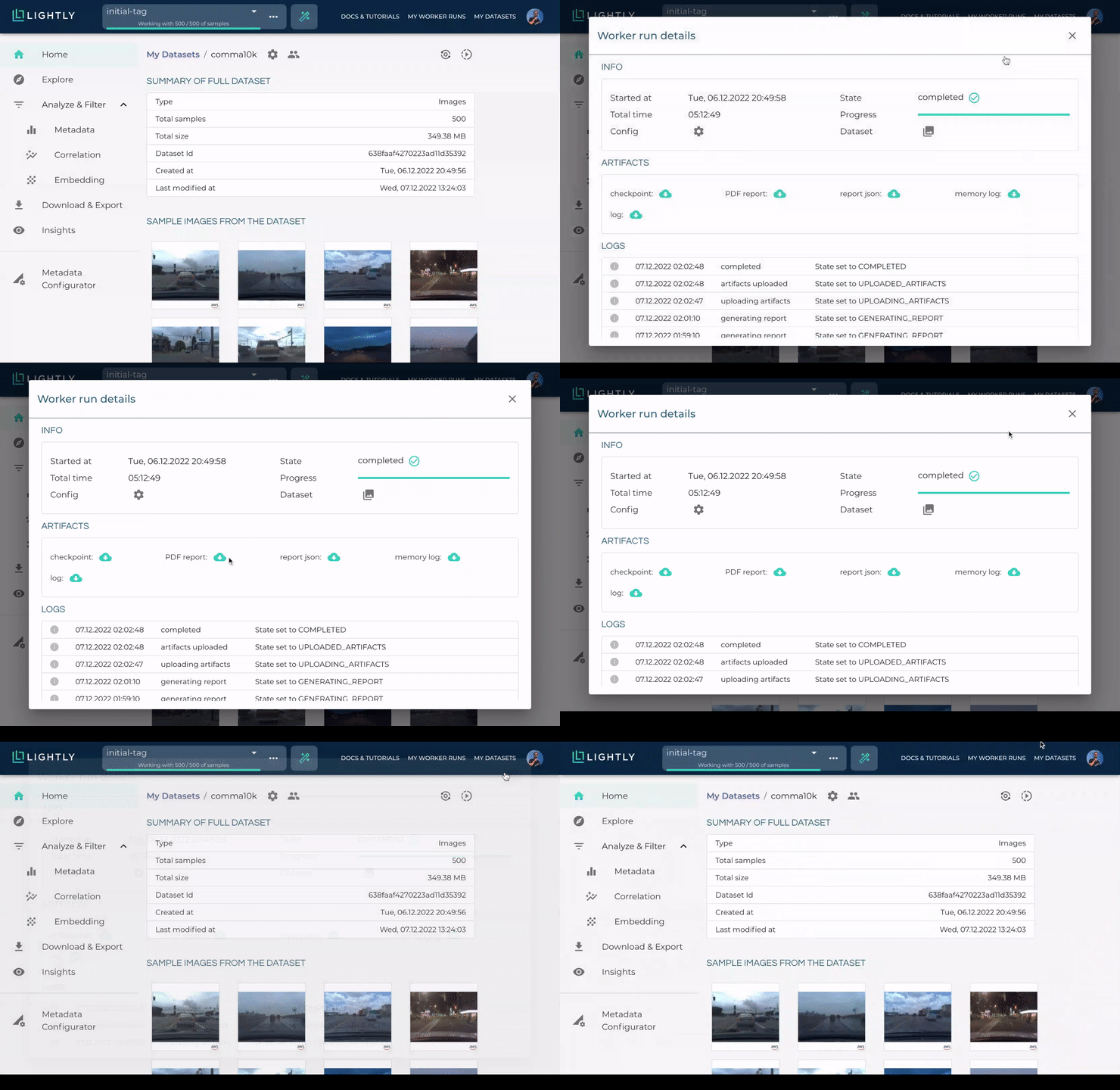
You can access the run artifacts either using code or through the user interface of the LightlyOne Platform.
The Dataset Filtering Report PDF
For every run, we also generate a PDF report summarizing what happened with the dataset before and after running it through the LightlyOne Solution. It's handy to have this in PDF form, as you might want to remove the unselected files from your bucket and won't have access to the images and statistics anymore afterward.
There are many plots and statistics in the PDF report. An interesting one for us is to see how the distribution of objects in the images changes through Lightly. If we would just randomly subsample the dataset, we would expect the distribution between input and output to stay the same.
However, our selection configuration has an impact on the balancing in several ways:
- We asked for diverse objects.
- We wanted a certain target distribution of the classes.
- We also wanted to prioritize images with more objects.
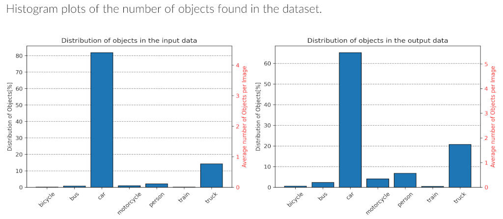
Using the LightlyOne selection configuration from above, were were able to not only find more diverse objects, but also rebalance the classes. Note that we heavily reduced the amount of cars from over 80% to about 65% while increasing objects of all of the other classes.
Exploring the Selected Data in the LightlyOne Platform
Using our interactive user interface, you can easily navigate through the selected data and get an overview before sending the data off to labeling.
Because we were using predictions and configured the LightlyOne Solution to select diverse objects, we will have not only the full-frame dataset in the Platform but also a second dataset solely consisting of the object crops.

If everything went as planned, you should see two datasets in the LightlyOne Platform. One for the full frame images and one for the crops of the object_detection_comma10k task.
The full frame dataset can be useful to see which 500 images have been selected and get a broad overview. You can spot some clusters such as different times of the day/night as well as weather conditions.
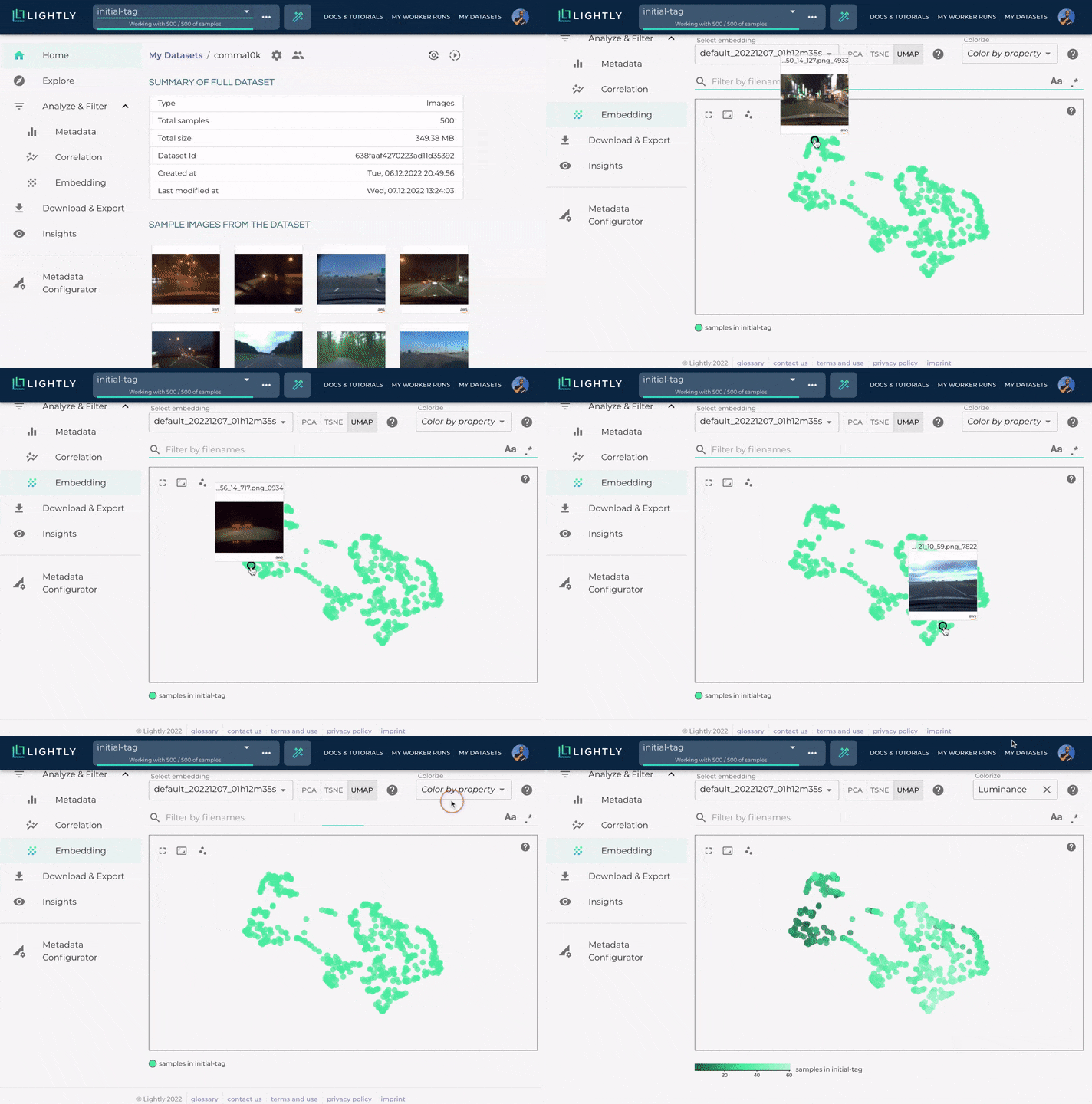
The LightlyOne Platform allows you to easily explore the selected data using the embeddings.
The crop dataset allows you to explore the data on a crop level. For each bounding box prediction, we crop out the object and compute the embedding. Since we still have access to the predicted class, we can also show the class label in the embedding view.
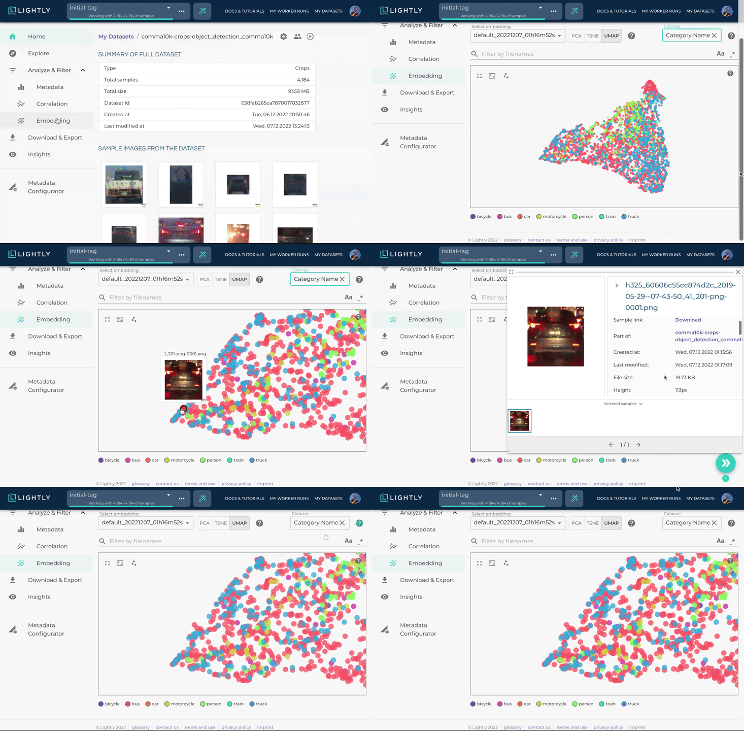
Explore the selected object crops using embeddings.
Export Filenames for Labeling
There are two ways of exporting data from Lightly. Either through the UI or (recommended by us) using the API.
Using the LightlyOne Python Client, this would work like this:
from lightly.api import ApiWorkflowClient

# Create the Lightly client to connect to the API.
# You can also combine this with the script above and reuse the client.
client = ApiWorkflowClient(token="MY_LIGHTLY_TOKEN", dataset_id="MY_DATASET_ID")

# get the filenames with signed read URLs
filenames_and_read_urls = client.export_filenames_and_read_urls_by_tag_name(
    tag_name="initial-tag"  # name of the tag in the dataset
)
with open("filenames-and-readurls-of-initial-tag.json", "w") as f:
    json.dump(filenames_and_read_urls, f)
In the UI, you can export the filenames using the Download & Export menu item.
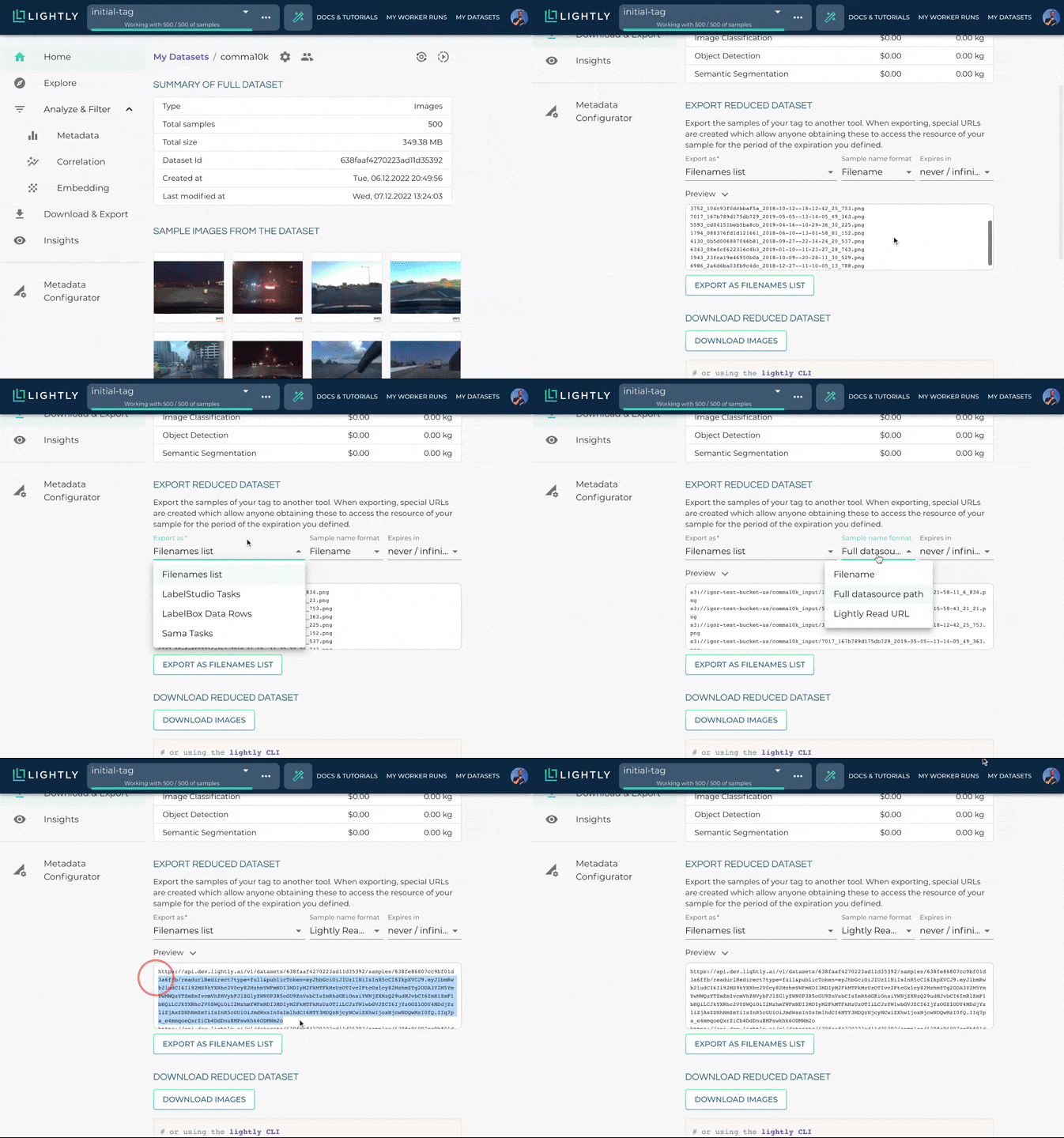
Export filenames through the UI.
Updated 7 months ago
